

Summer is just around the corner and everybody seems to be asking the same question: “does my data look... out of shape?” Whether you’re a scientist or an engineer, data-image dysmorphia can lead to serious negative thoughts which leave you second-guessing our data.
Much has already been said about modifying DataFrames on a “micro” level, such as column-wise operations. But what about modifying entire DataFrames at once? When considering Numpy’s role in general mathematics, it should come as no surprise that Pandas DataFrames have a lot of similarities to the matrices we learned high school pre-calc; namely, they like to be changed all at once. It’s easy to see this in action when applying basic math functions to multiple DataFrames like df1 + df2, df1 / df2, etc.
Aside from weapons of math destruction, there are plenty of ways to act on entire tables of data. We might do this for a number of reasons such as preparing data for data visualization, or to reveal the secrets hidden within. This sounds harder than it is in practice. Modifying data in this manner is surprisingly easy, and most of the terminology we’ll cover will sound familiar to a typical spreadsheet junkie. The challenge is knowing when to use these operations, and a lot of that legwork is covered by simply knowing that they exist. I was lucky enough to have learned this lesson from my life mentor: GI Joe.
I’ll be demonstrating these operations in action using StackOverflow’s 2018 developer survey results. I’ve already done some initial data manipulation to save you from the boring stuff. Here’s a peek at the data:
| Respondent | Country | OpenSource | Employment | HopeFiveYears | YearsCoding | CurrencySymbol | Salary | FrameworkWorkedWith | Age | Bash/Shell | C | C++ | Erlang | Go | Java | JavaScript | Objective-C | PHP | Python | R | Ruby | Rust | SQL | Scala | Swift | TypeScript |
|---|---|---|---|---|---|---|---|---|---|---|---|---|---|---|---|---|---|---|---|---|---|---|---|---|---|---|
| 3 | United Kingdom | Yes | Employed full-time | Working in a different or more specialized technical role than the one I'm in now | 30 or more years | GBP | 51000.0 | Django | 35 - 44 years old | 1 | 0 | 0 | 0 | 0 | 0 | 1 | 0 | 0 | 1 | 0 | 0 | 0 | 0 | 0 | 0 | 0 |
| 7 | South Africa | No | Employed full-time | Working in a different or more specialized technical role than the one I'm in now | 6-8 years | ZAR | 260000.0 | 18 - 24 years old | 1 | 1 | 1 | 0 | 0 | 1 | 0 | 0 | 0 | 0 | 1 | 0 | 0 | 1 | 0 | 0 | 0 | |
| 8 | United Kingdom | No | Employed full-time | Working in a different or more specialized technical role than the one I'm in now | 6-8 years | GBP | 30000.0 | Angular;Node.js | 18 - 24 years old | 0 | 0 | 0 | 0 | 0 | 1 | 1 | 0 | 0 | 1 | 0 | 0 | 0 | 0 | 0 | 0 | 1 |
| 9 | United States | Yes | Employed full-time | Working as a founder or co-founder of my own company | 9-11 years | USD | 120000.0 | Node.js;React | 18 - 24 years old | 0 | 0 | 0 | 0 | 0 | 0 | 1 | 0 | 0 | 0 | 0 | 0 | 0 | 0 | 0 | 0 | 0 |
| 11 | United States | Yes | Employed full-time | Doing the same work | 30 or more years | USD | 250000.0 | Hadoop;Node.js;React;Spark | 35 - 44 years old | 1 | 0 | 0 | 1 | 1 | 0 | 1 | 0 | 0 | 1 | 0 | 1 | 0 | 1 | 0 | 0 | 0 |
| 21 | Netherlands | No | Employed full-time | Working in a career completely unrelated to software development | 0-2 years | EUR | 0.0 | 18 - 24 years old | 0 | 0 | 0 | 0 | 0 | 1 | 1 | 0 | 1 | 0 | 0 | 0 | 0 | 0 | 0 | 0 | 0 | |
| 27 | Sweden | No | Employed full-time | Working in a different or more specialized technical role than the one I'm in now | 6-8 years | SEK | 32000.0 | .NET Core | 35 - 44 years old | 1 | 0 | 0 | 0 | 0 | 0 | 0 | 0 | 0 | 0 | 0 | 0 | 0 | 1 | 0 | 0 | 0 |
| 33 | Australia | Yes | Employed full-time | Working in a different or more specialized technical role than the one I'm in now | 15-17 years | AUD | 120000.0 | Angular;Node.js | 35 - 44 years old | 0 | 1 | 1 | 0 | 1 | 0 | 0 | 0 | 0 | 1 | 0 | 0 | 0 | 1 | 0 | 1 | 0 |
| 37 | United Kingdom | No | Employed full-time | Working as a product manager or project manager | 9-11 years | GBP | 25.0 | .NET Core | 25 - 34 years old | 0 | 0 | 0 | 0 | 0 | 0 | 1 | 0 | 1 | 0 | 0 | 0 | 0 | 1 | 0 | 0 | 0 |
| 38 | United States | No | Employed full-time | Working in a career completely unrelated to software development | 18-20 years | USD | 75000.0 | 45 - 54 years old | 1 | 0 | 0 | 0 | 0 | 0 | 1 | 0 | 1 | 0 | 0 | 0 | 0 | 1 | 0 | 0 | 0 |
<class 'pandas.core.frame.DataFrame'>
Int64Index: 49236 entries, 1 to 89965
Data columns (total 27 columns):
Respondent             49236 non-null int64
Country                49236 non-null object
OpenSource             49236 non-null object
Employment             49066 non-null object
HopeFiveYears          48248 non-null object
YearsCoding            49220 non-null object
CurrencySymbol         48795 non-null object
Salary                 48990 non-null float64
FrameworkWorkedWith    34461 non-null object
Age                    47277 non-null object
Bash/Shell             49236 non-null uint8
C                      49236 non-null uint8
C++                    49236 non-null uint8
Erlang                 49236 non-null uint8
Go                     49236 non-null uint8
Java                   49236 non-null uint8
JavaScript             49236 non-null uint8
...
dtypes: float64(1), int64(1), object(8), uint8(17)
memory usage: 6.2+ MBstackoverflow_df.info()Group By
You’re probably already familiar with the modest groupby() method, which allows us to perform aggregate functions on our data. groupby() is critical for gaining a high-level insight into our data or extracting meaningful conclusions.
Let's check out how our data is distributed. Let's see the general age range of people who took the StackOverflow interview. I'm going to reduce our DataFrame into two columns first:
# Remove columns
grouped_df = stackoverflow_df.filter(
    items=[
        'Country',
        'Age'
    ]
)

# Aggregate by age
grouped_df = grouped_df.groupby(['Age']).count()groupby() methodWe use count() to specify the aggregate type. In this case, count() will give us the number of times each value occurs in our data set:
                    Country
Age
18 - 24 years old      9840
25 - 34 years old     25117
35 - 44 years old      8847
45 - 54 years old      2340
55 - 64 years old       593
65 years or older        73
Under 18 years old 467print(grouped_df)Cool, looks like there's a lot of us over the age of 25! Screw those young guys.
Why are our values stored under the county column (what exactly does Country = 25117 mean)? When we aggregate by count, non-grouped columns have their values replaced with the count of our grouped column... which is pretty confusing. If we had left all columns in before performing groupby(), all columns would have contained these same values. That isn't very useful.
Just for fun, let's build on this to find the median salary per age group:
# Remove columns
grouped_df = stackoverflow_df.filter(
    items=[
        'Salary',
        'Age',
        'CurrencySymbol'
    ]
)

# Get median salary by age
grouped_df = grouped_df.loc[groupedDF['CurrencySymbol'] == 'USD']
grouped_df = grouped_df.groupby(['Age']).median()

# Sort descending
grouped_df.sort_values(
    by=['Salary'],
    inplace=True,
    ascending=False
)median aggregation to discern pay median by age rangeLet's have a look:
                      Salary
Age
45 - 54 years old   120000.0
55 - 64 years old   120000.0
35 - 44 years old   110000.0
65 years or older    99000.0
25 - 34 years old    83000.0
18 - 24 years old    50000.0
Under 18 years old 0.0print(grouped_df)Melt
I'm not sure if you noticed earlier, but our data set is a little weird. There's a column for each programming language in existence, which makes our table exceptionally long. Who would do such a thing? (I did, for demonstration purposes tbh). Scroll sideways below for a look (sorry Medium readers):
| Respondent | Country | OpenSource | Employment | HopeFiveYears | YearsCoding | CurrencySymbol | Salary | FrameworkWorkedWith | Age | Bash/Shell | C | C++ | Erlang | Go | Java | JavaScript | Objective-C | PHP | Python | R | Ruby | Rust | SQL | Scala | Swift | TypeScript |
|---|---|---|---|---|---|---|---|---|---|---|---|---|---|---|---|---|---|---|---|---|---|---|---|---|---|---|
| 3 | United Kingdom | Yes | Employed full-time | Working in a different or more specialized technical role than the one I'm in now | 30 or more years | GBP | 51000.0 | Django | 35 - 44 years old | 1 | 0 | 0 | 0 | 0 | 0 | 1 | 0 | 0 | 1 | 0 | 0 | 0 | 0 | 0 | 0 | 0 |
| 7 | South Africa | No | Employed full-time | Working in a different or more specialized technical role than the one I'm in now | 6-8 years | ZAR | 260000.0 | 18 - 24 years old | 1 | 1 | 1 | 0 | 0 | 1 | 0 | 0 | 0 | 0 | 1 | 0 | 0 | 1 | 0 | 0 | 0 | |
| 8 | United Kingdom | No | Employed full-time | Working in a different or more specialized technical role than the one I'm in now | 6-8 years | GBP | 30000.0 | Angular;Node.js | 18 - 24 years old | 0 | 0 | 0 | 0 | 0 | 1 | 1 | 0 | 0 | 1 | 0 | 0 | 0 | 0 | 0 | 0 | 1 |
| 9 | United States | Yes | Employed full-time | Working as a founder or co-founder of my own company | 9-11 years | USD | 120000.0 | Node.js;React | 18 - 24 years old | 0 | 0 | 0 | 0 | 0 | 0 | 1 | 0 | 0 | 0 | 0 | 0 | 0 | 0 | 0 | 0 | 0 |
| 11 | United States | Yes | Employed full-time | Doing the same work | 30 or more years | USD | 250000.0 | Hadoop;Node.js;React;Spark | 35 - 44 years old | 1 | 0 | 0 | 1 | 1 | 0 | 1 | 0 | 0 | 1 | 0 | 1 | 0 | 1 | 0 | 0 | 0 |
That's a lot of nonsense! A good way to handle data split out like this is by using Pandas' melt(). In short, melt() takes values across multiple columns and condenses them into a single column. In the process, every row of our DataFrame will be duplicated a number of times equal to the number of columns we're "melting". It's easier to communicate this visually:
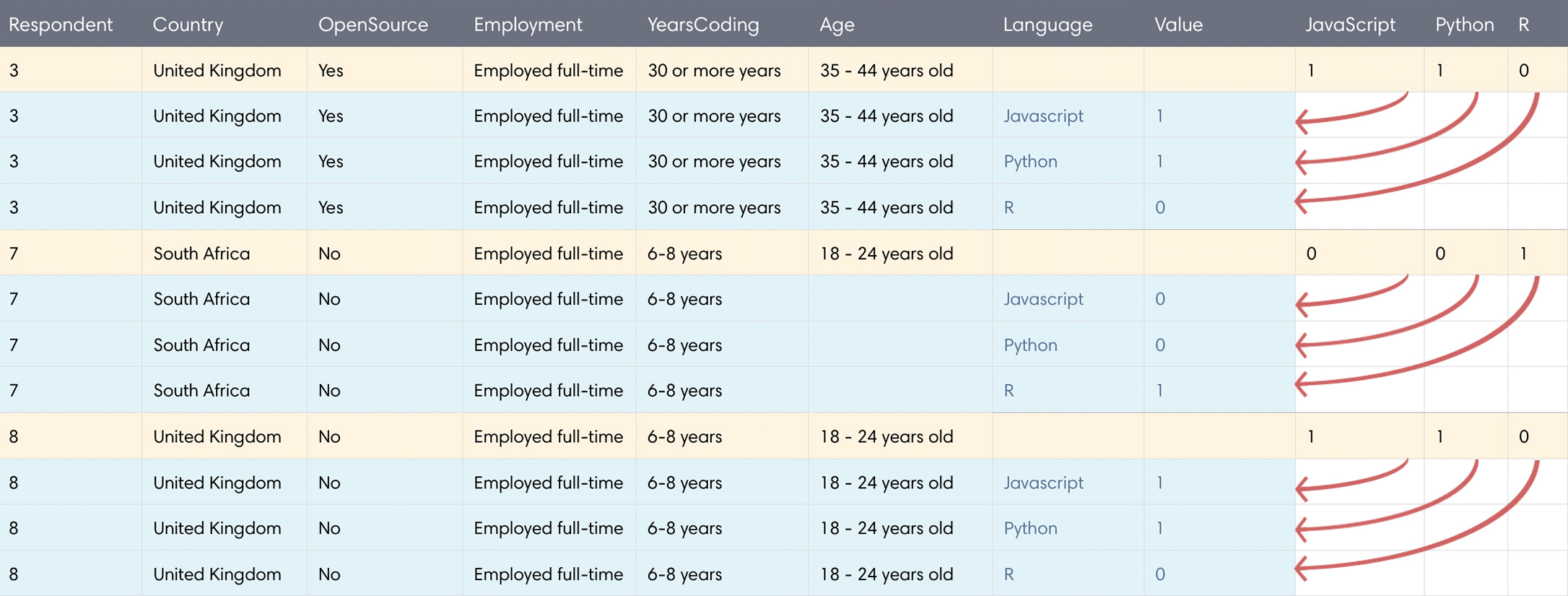
melt()In the above example, we're using melt() on a sample size of 3 rows (yellow) and 3 columns (JavaScript, Python, R). Each melted column name is moved under a new column called Language. For each column we melt, an existing row is duplicated to accommodate tucking data into a single column and our DataFrame grows longer. We're melting 3 columns in the example above, thus each original rows gets duplicated 3 times (new rows displayed in blue). Our sample of 3 rows turns into 9 total, and our 3 melted columns go away. Let's see it in action:
melt_df = pd.melt(stackoverflow_df,
                 id_vars=['Respondent',
                          'Country',
                          'OpenSource',
                          'Employment',
                          'HopeFiveYears',
                          'YearsCoding',
                          'CurrencySymbol',
                          'Salary'],
                  value_vars=['JavaScript',
                              'Python',
                              'Go',
                              'Java',
                              'Objective-C',
                              'Swift',
                              'R',
                              'Ruby',
                              'Rust',
                              'SQL',
                              'Scala',
                              'PHP'],
                  var_name='Language')
melt() columns representing programming languagesid_vars are the columns we keep the same which will be melted into. value_vars are the columns we'd like to melt. Lastly, we name our new column of consolidated values with var_name. Here's what .info() looks like after we run this:
<class 'pandas.core.frame.DataFrame'>
RangeIndex: 590832 entries, 0 to 590831
Data columns (total 10 columns):
Respondent        590832 non-null int64

Country           590832 non-null object
OpenSource        590832 non-null object
Employment        588792 non-null object
HopeFiveYears     578976 non-null object
YearsCoding       590640 non-null object
CurrencySymbol    585540 non-null object
Salary            587880 non-null float64
Language          590832 non-null object
value             590832 non-null int64
dtypes: float64(1), int64(2), object(7)
memory usage: 45.1+ MBprint(melt_df.info())The visual effect of this is that wide DataFrames become very, very long (our memory usage went from 6.2mb to 45.1mb!). Why is this useful? For one, what happens if a new programming language is invented? If this happens often, it's probably best not to have these split into columns. Even more importantly, this format is essential for tasks such as charting data (like we saw in the Seaborn tutorial), or creating pivot tables.
Combing melt() with groupby()
With our data melted, it's way easier to extract information using groupby(). Let's figure out the most commonly known programming languages! To do this, I'll take our DataFrame and make the following adjustments:
- Remove the extra columns.
- Drop rows where language value is 0.
- Perform a
sum()aggregate.
melt_df.drop(columns=['Respondent', 'Salary'], inplace=True)
melt_df = melt_df.loc[melt_df['value'] == 1]

# Group by the aggregate sum of language usage
melt_df = melt_df.groupby(['Language']).sum()

# Sort by language popularity
melt_df.sort_values(
    by=['value'],
    inplace=True,
    ascending=False
)melt() with groupby()And the output...
Language
JavaScript   35736
SQL          29382
Java         21451
Python       19182
PHP          14644
Ruby          5512
Swift         4037
Go            3817
Objective-C   3536
R 3036print(meltDF.head(10))Pivot Tables
Pivot tables allow us to view aggregates across two dimensions. In the aggregation we performed above, we found the overall popularity of programming languages (1-dimensional aggregate). To image what a 2-dimensional aggregate looks like, we'll expand on this example to split our programming language totals into a second dimension: popularity by age group.
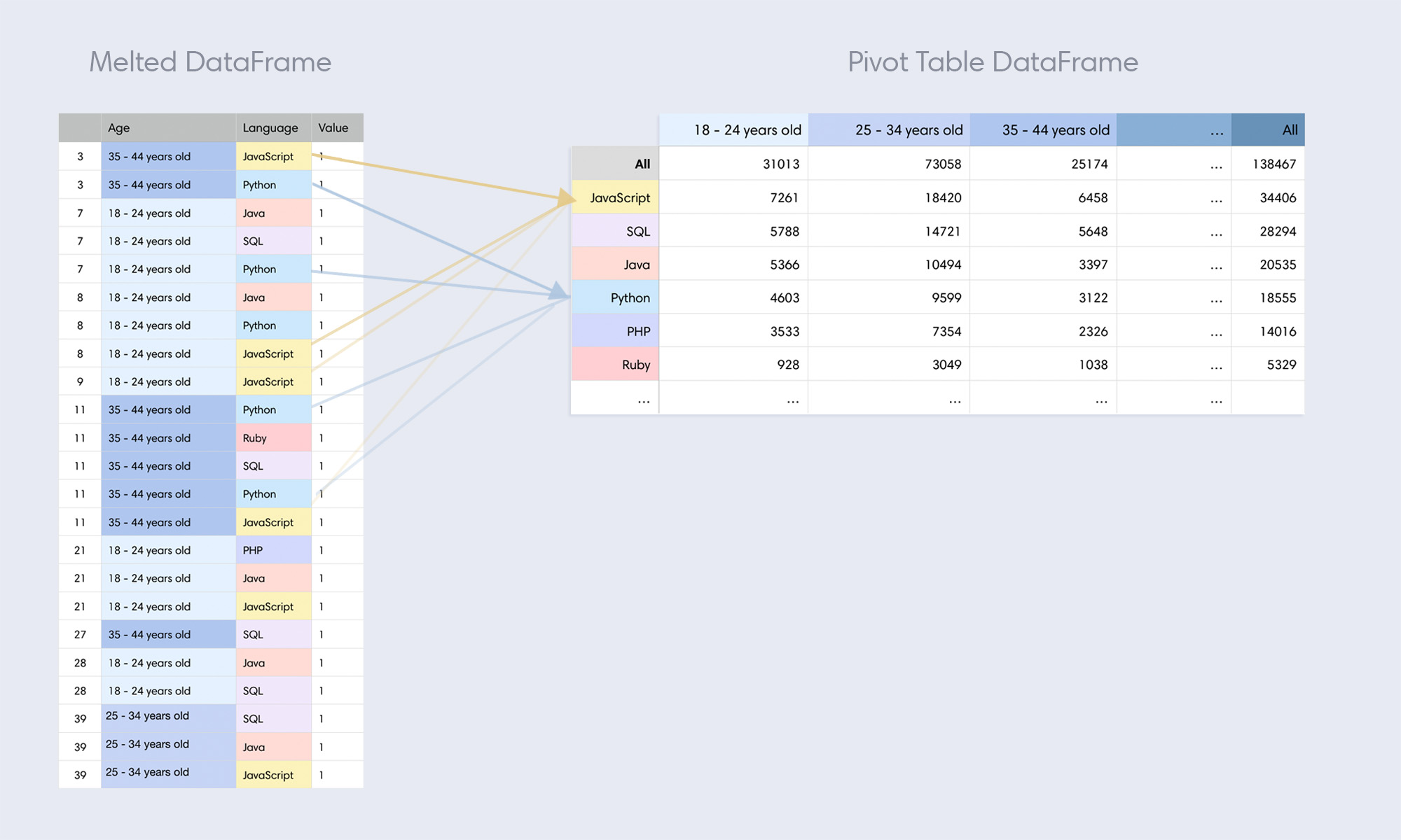
On the left is our melted DataFrame reduced to three columns: Age, Language, and Value (I've also shown the Respondent ID column for reference). When we create a Pivot table, we take the values in one of these two columns and declare those to be columns in our new table (notice how the values in Age on the left become columns on the right). When we do this, the Language column becomes what Pandas calls the 'id' of the pivot (identifier by row).
Our pivot table only contains a single occurrence of the values we use in our melted DataFrame (JavaScript appears many times on the left, but once on the right). Every time we create a pivot table, we're aggregating the values in two columns and splitting them out two-dimensionally. The difference between a pivot table and a regular pivot is that pivot tables always perform an aggregate function, whereas plain pivots do not.
Our pivot table now shows language popularity by age range. This can give us some interesting insights, like how Java is more popular in kids under the age of 25 than Python (somebody needs to set these kids straight).
Here's how we do this in Pandas:
# Keep relevent columns
pivot_table_df = stackoverflow_df.filter(
    items=[
        'Age',
        'Language',
        'value'
    ]
)

# Create pivot table
pivot_table_df = pd.pivot_table(
    stackoverflow_df,
    index='Language',
    columns='Age',
    values='value',
    aggfunc=np.sum,
    margins=True
)

# Sort table
pivot_table_df.sort_values(
    by=['All'],
    inplace=True,
    ascending=False
)pd.pivot_table() is what we need to create a pivot table (notice how this is a Pandas function, not a DataFrame method). The first thing we pass is the DataFrame we'd like to pivot. Then are the keyword arguments:
- index: Determines the column to use as the row labels for our pivot table.
- columns: The original column which contains the values which will make up new columns in our pivot table.
- values: Data which will populate the cross-section of our index rows vs columns.
- aggfunc: The type of aggregation to perform on the values we'll show. count would give us the number of occurrences, mean would take an average, and median would... well, you get it (for my own curiosity, I used median to generate some information about salary distribution... try it out).
- margins: Creates a column of totals (named "All").
Transpose
Now this is the story all about how my life got flipped, turned upside down. That's what you'd be saying if you happened to be a DataFrame which just got transposed.
Transposing a DataFrame simply flips a table on its side, so that rows become columns and vice versa. Here's an awful idea: let's try this on our raw data!:
# Keep relevent columns
stackoverflow_df = stackoverflow_df.filter(
    items=[
        'Respondent',
        'Country',
        'OpenSource',
        'Employment',
        'HopeFiveYears',
        'YearsCoding',
        'CurrencySymbol',
        'Salary',
        'Age'
    ]
)

# Flip our DataFrame
stackoverflow_df = stackoverflow_df.transpose()transpose()Transposing a DataFrame is as simple as df.transpose(). The outcome is exactly what we'd expect:
| FIELD1 | 0 | 1 | 2 | 3 | 4 |
|---|---|---|---|---|---|
| Respondent | 3 | 7 | 8 | 9 | 11 |
| Country | United Kingdom | South Africa | United Kingdom | United States | United States |
| OpenSource | Yes | No | No | Yes | Yes |
| Employment | Employed full-time | Employed full-time | Employed full-time | Employed full-time | Employed full-time |
| HopeFiveYears | Working in a different or more specialized technical role than the one I'm in now | Working in a different or more specialized technical role than the one I'm in now | Working in a different or more specialized technical role than the one I'm in now | Working as a founder or co-founder of my own company | Doing the same work |
| YearsCoding | 30 or more years | 6-8 years | 6-8 years | 9-11 years | 30 or more years |
| CurrencySymbol | GBP | ZAR | GBP | USD | USD |
| Salary | 51000.0 | 260000.0 | 30000.0 | 120000.0 | 250000.0 |
| Age | 35 - 44 years old | 18 - 24 years old | 18 - 24 years old | 18 - 24 years old | 35 - 44 years old |
Of course, those are just the first 5 columns. The actual shape of our DataFrame is now [9 rows x 49236 columns]. Admittedly, this wasn't the best example.
Stack and Unstack
Have you ever run into a mobile-friendly responsive table on the web? When viewing tabular data on a mobile device, some sites present data in a compact "stacked" format, which fits nicely on screens with limited horizontal space. That's the best way I can describe what stack() does, but see for yourself:
stackoverflow_df = stackoverflow_df.stack()stack() methodThe output:
0  Respondent                                                        3
   Country                                              United Kingdom
   OpenSource                                                      Yes
   Employment                                       Employed full-time
   HopeFiveYears     Working in a different or more specialized tec...
   YearsCoding                                        30 or more years
   CurrencySymbol                                                  GBP

   Salary                                                        51000
   Age                                               35 - 44 years old
1  Respondent                                                        7
   Country                                                South Africa
   OpenSource                                                       No
   Employment                                       Employed full-time
   HopeFiveYears     Working in a different or more specialized tec...
   YearsCoding                                               6-8 years
   CurrencySymbol                                                  ZAR
   Salary                                                       260000
   Age                                               18 - 24 years old
2  Respondent                                                        8
   Country                                              United Kingdom
   OpenSource                                                       No
   Employment                                       Employed full-time
   HopeFiveYears     Working in a different or more specialized tec...
   YearsCoding                                               6-8 years
   CurrencySymbol                                                  GBP
   Salary                                                        30000
   Age                                               18 - 24 years old
3  Respondent                                                        9
   Country                                               United States
   OpenSource                                                      Yes
   Employment                                       Employed full-time
   HopeFiveYears     Working as a founder or co-founder of my own c...
   YearsCoding                                              9-11 years
   CurrencySymbol                                                  USD
   Salary                                                       120000
   Age                                               18 - 24 years old
...print(stackoverflow_df)Our data is now "stacked" according to our index. See what I mean? Stacking supports multiple indexes as well, which can be passed using the level keyword parameter.
To undo a stack, simply use df.unstack().
Anyway, I'm sure you're eager to hit the beach and show off your shredded data. I'll let you get to it. You've earned it.