

I've been wandering into a lot of awkward conversations lately, most of them being about how I spend my free time. Apparently "rifling through Python library documentation in hopes of finding dope features" isn't considered a relatable hobby by most people. At least you're here, so I must be doing something right occasionally.
Today we'll be venturing off into the world of Pandas indexes. Not just any old indexes... hierarchical indexes. Hierarchical indexes take the idea of having identifiers for rows, and extends this concept by allowing us to set multiple identifiers with a twist: these indexes hold parent/child relationships to one another. These relationships enable us to do cool things like instantly organize our data into groups without performing groupbys. When used correctly, these relationships can be immensely helpful when we need to do some really powerful analysis.
Hierarchical indexes (AKA multiindexes) help us to organize, find, and aggregate information faster at almost no cost. Organizing data in this way is super cool, but also quite tricky to get the hang of at first. We'll take it one step at a time.
Creating a DataFrame With a Hierarchical Index
There are many ways to declare multiple indexes on a DataFrame - probably way more than you'll ever need. The most straightforward approach is just like setting a single index; we pass an array of columns to index= instead of a string!
To demonstrate the art of indexing, we're going to use a dataset containing a few years of NHL game data. Let's load it up:
import pandas as pd
nhlDF = pd.read_csv('data/nhl.csv')
nhlDF['date'] = pd.to_datetime(nhlDF['date'])
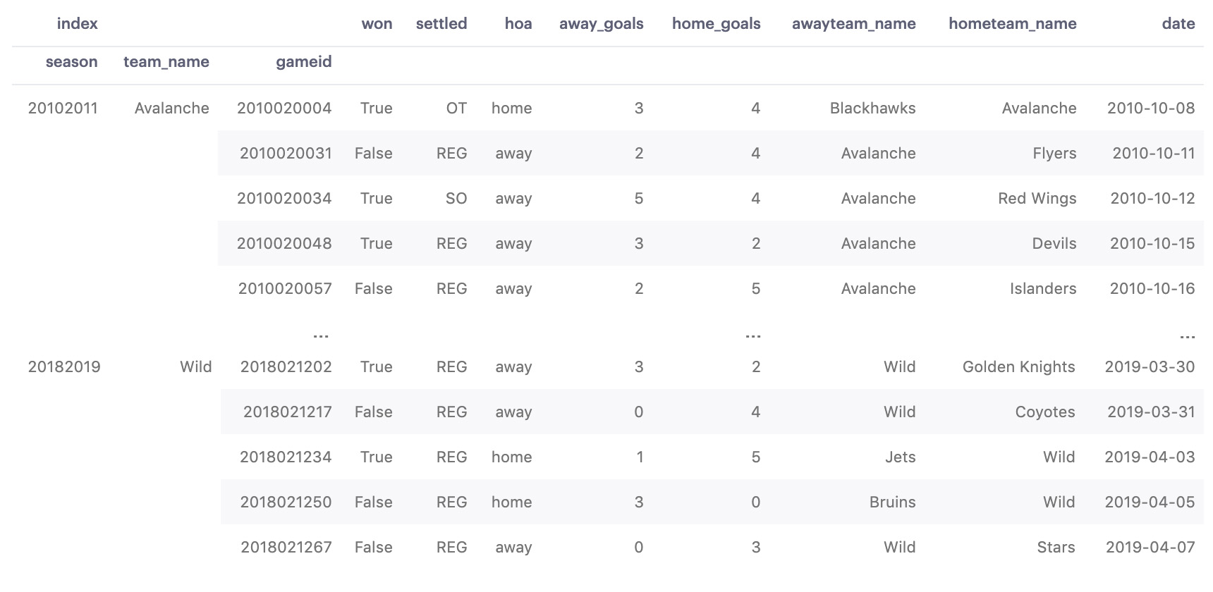
print(nhlDF.head(5))
print(nhlDF.tail(5))| season | team_name | game_id | won | settled | hoa | away_goals | home_goals | awayteam_name | hometeam_name | date |
|---|---|---|---|---|---|---|---|---|---|---|
| 20102011 | Avalanche | 2010020004 | TRUE | OT | home | 3 | 4 | Blackhawks | Avalanche | October 8, 2010 |
| 20102011 | Avalanche | 2010020031 | FALSE | REG | away | 2 | 4 | Avalanche | Flyers | October 11, 2010 |
| 20102011 | Avalanche | 2010020034 | TRUE | SO | away | 5 | 4 | Avalanche | Red Wings | October 12, 2010 |
| 20102011 | Avalanche | 2010020048 | TRUE | REG | away | 3 | 2 | Avalanche | Devils | October 15, 2010 |
| 20102011 | Avalanche | 2010020057 | FALSE | REG | away | 2 | 5 | Avalanche | Islanders | October 16, 2010 |
| 20182019 | Wild | 2018021202 | TRUE | REG | away | 3 | 2 | Wild | Golden Knights | March 30, 2019 |
| 20182019 | Wild | 2018021217 | FALSE | REG | away | 0 | 4 | Wild | Coyotes | March 31, 2019 |
| 20182019 | Wild | 2018021234 | TRUE | REG | home | 1 | 5 | Jets | Wild | April 3, 2019 |
| 20182019 | Wild | 2018021250 | FALSE | REG | home | 3 | 0 | Bruins | Wild | April 5, 2019 |
| 20182019 | Wild | 2018021267 | FALSE | REG | away | 0 | 3 | Wild | Stars | April 7, 2019 |
Each row in our dataset contains information regarding the outcome of a hockey match. We have a row called season, with values such as 20102011. This integer represents the NHL season in which the game was played (in this example, 20102011 refers to the 2010-2011 season). We also have columns such as team_name and game_idsuccess with hierarchical indexes is first considering how we want to look at our data, which are fine index candidates.
The key to success with hierarchical indexes is to first consider how we want to look at our data and which questions we're trying to answer. Off the bat, I already know that I will be looking at this data by drilling into the seasonGames determine a team's performance first: teams change drastically from season to season, and I'm more interested to see how our teams did on a per-season basis than a period of 8 years. Next, I will organize our data by team_name to see Team X's performance in a given season. Games determine a team's performance; thus game_id will be our third and final index.
Here's how we'd set that index:
# Create Multiindex
nhl_df.set_index(['season', 'team_name', 'game_id'], inplace=True)
nhl_df.sort_index(inplace=True)

# Print a preview of our data
print(nhl_df.head(5))
print(nhlDF.tail(5))
Setting a 3-tier index on a DataFrame and view the results
Let's see how things have changed:
Our data already looks more organized, but there's more to multiindexes than looks. We've created a hierarchy of relationships in our data! With these indexes, we've silently made small distinctions in our data. For instance, we've distinguished that the Golden Knights of 2018-2019 are a different entity than the Golden Knights, which made it to the Stanley Cup in the 2017-2018 season. We also associated all the games played by the Golden Knights this season t0 this season's Golden Knights, which is, in turn, a child of 2018-2019. As a result, we've gained insight into which season each game belongs to.
While this hierarchy of indexes is in place, the information stored across all 3 indexes is inseparable from the values in each row. I'll show you what I mean.
2D Series
Let's look at a series in our newly indexed data. You know all about Pandas' Series datatype: they're nicely keyed columns of data without any funny business:
# Demonstrate 2D Series
print(nhl_df['date'].head(10))
View the dates of the first 10 entries in our date column
season    team_name  game_id
20102011  Avalanche  2010020004   2010-10-08
                     2010020031   2010-10-11
                     2010020034   2010-10-12
                     2010020048   2010-10-15
                     2010020057   2010-10-16
                     2010020070   2010-10-18
                     2010020090   2010-10-22
                     2010020108   2010-10-24
                     2010020122   2010-10-27
                     2010020136   2010-10-29
Name: date, dtype: datetime64[ns]
Whoa, what's all this funny business?! We printed a single column with nhl_df['date'], so what's with the 4-columns?
As mentioned earlier, the relationships we create with hierarchical indexes make these relationships inseparable: no matter how we mess with our data, the indexes will follow. In essence, this makes our series 2-dimensional. This is really cool because we can manipulate our series as normal ( nhl_df['date'][0] still gets us the first value, etc.), but now we have associated metadata about each row.
MultiIndex.from_arrays and MultiIndex.from_tuples which gives us some flexibility, but I personally have no interest in boring anybody with these. If you're feeling bored, read the docs.Inspecting and Modifying DataFrame Indexes
Before we get too crazy, let's quickly cover a few fundamental multiindex bases. Check out what happens when we inspect the indexes on our DataFrame:
# Inspect indexes
print(nhl_df.index)
Viewing the indexes of a multi-index DataFrame
Output:
MultiIndex(levels=[[20102011, 20112012, 20122013, 20132014, 20142015, ...],
                   ['Avalanche', 'Blackhawks', 'Blue Jackets', ...],
                   [2010020001, 2010020002, 2010020003, 2010020004, ...]],
           labels=[[0, 0, 0, 0, 0, 0, 0, 0, 0, 0, 0, 0, 0, 0, ...]],
           names=['season', 'team_name', 'game_id'])
The output of viewing a multi-indexed DataFrame
A wild MultiIndex appears! In Pandas, MultiIndex is a datatype in itself. This can be useful if you need to deal with creating indexes with highly complex logic dynamically. It's pretty cool that we can rip the indexing scheme out of any DataFrame, as well as pass that scheme into a new DataFrame.
I've truncated the values returned by print(nhl_df.index) to avoid pasting thousands of results. Let's break this down. The names attribute reiterates our hierarchical structure: ['season', 'team_name', 'game_id']. We also see the values of our indexes being populated into levels.
A level refers to the name of one of the indexes in our hierarchy. Our left-most index is our highest-level index and can be referred to as level 0. In our example, season is level 0. Levels can also be referred to by their name, thus level=0 is interchangeable with level='season'. Modifying levels has the same syntax as working with columns.
Let's look at our index values tho:
# Inspect index values
print(nhlDF.index.values)
[(20102011, 'Avalanche', 2010020004) (20102011, 'Avalanche', 2010020031)
(20102011, 'Avalanche', 2010020034) ... (20182019, 'Wild', 2018021234)
(20182019, 'Wild', 2018021250) (20182019, 'Wild', 2018021267)]Oh snap, tuples! Generally speaking, hierarchical indexes like to be tossed around as tuple values. Not really useful for now, but maybe for later.
Sorting Data by Index
You may have noticed that I blew past nhl_df.sort_index(inplace=True) when we created our indexes. Sorting our index is very important after setting a hierarchical index; if we hadn't done so, selecting and aggregating our data could actually result in errors. If we consider the way indexes are "grouped," it makes sense as to why this would happen: how can we group our data in a visually pleasing way if it's still scattered everywhere?
Resetting Indexes
Remember that columns and indexes are not the same, even if they may seem similar. When a column becomes an index, the original "column" is dropped, and an index is added to our DataFrame with the values that were contained in said column. While we still have values for season, team_name, and game_id, our DataFrame is technically 3 columns shorter than our original import. What have I done?! Does this mean I secretly destroyed the dataset you've been following along with? How could I!
Chill. Everything we've done thus far can be immediately undone at any time using nhlDF.reset_index(inplace=True). Resetting the index on a multiindex DataFrame unstacks our data and re-adds the original columns.
It's worth considering how powerful this can be if used correctly. I was able to index 22,694 rows on a free cluster in the blink of an eye and can disregard this just as quickly and easily. If we wanted, we could gun-sling DataFrame indexes all we want just for the purpose of answering a few questions, and revert back whenever we wanted. Let's see how these indexes might help us solve such questions.
Other Index Modifications
There's more we can do with index customization. Picking up on the usefulness of these things comes with a bit of time (and StackOverflow), but it doesn't hurt to know about these:
- Swap Index Levels:
df.swaplevel(i='level_name_1', j='level_name_2') - Rename Indexes:
df.index.names = ['name1', 'name2'] - Remove a single index level:
df.unstack(level=0)
Selecting Data in a Hierarchical Index
Now we can start doing something worthwhile. Let's see how using hierarchical indexes can help us find the data we're looking for.
Using .loc()
It's our good friend .loc()! Let's use .loc() to find all games in the 2010-2011 season:
# Select 2010-2011 season using iloc
print(nhl_df.loc[20102011, :].head(10))
Using the .loc() method to find games in a given season.
We're searching for instances of 20102011 here. We pass : to specify "all columns" for each row matched. If we wanted, we could replace : with column labels to find "all values in [columns] where row label is 20102011".
| team_name | won | away_goals | home_goals |
|---|---|---|---|
| Lightning | 62 | 260 | 287 |
| Flames | 50 | 250 | 266 |
| Bruins | 49 | 219 | 255 |
| Islanders | 48 | 206 | 218 |
| Capitals | 48 | 252 | 275 |
| Predators | 47 | 220 | 234 |
| Jets | 47 | 239 | 277 |
| Blue Jackets | 47 | 250 | 240 |
| Sharks | 46 | 260 | 290 |
| Hurricanes | 46 | 225 | 243 |
| Maple Leafs | 46 | 263 | 274 |
| Blues | 45 | 234 | 236 |
| Canadiens | 44 | 223 | 262 |
| Penguins | 44 | 263 | 251 |
| Stars | 43 | 186 | 226 |
| Golden Knights | 43 | 218 | 261 |
| Coyotes | 39 | 203 | 233 |
| Avalanche | 38 | 245 | 261 |
| Flyers | 37 | 258 | 267 |
| Wild | 37 | 225 | 223 |
| Blackhawks | 36 | 268 | 294 |
| Panthers | 36 | 250 | 297 |
| Oilers | 35 | 241 | 265 |
| Ducks | 35 | 207 | 243 |
| Canucks | 35 | 229 | 250 |
| Sabres | 33 | 233 | 264 |
| Rangers | 32 | 228 | 271 |
| Red Wings | 32 | 239 | 265 |
| Kings | 31 | 222 | 243 |
| Devils | 31 | 218 | 279 |
| Senators | 29 | 242 | 302 |
Boom. Those are all the games in 2010-2011. Notice how our season index appears to be missing? When we select and/or aggregate into an index, the level of index we're working against is omitted from the result to avoid being redundant.
Using .xs()
.xs() stands for cross section: it accepts a value to be found in an index, allowing for easier selection of rows by index. The below snippet will yield the same result as what we accomplished with .loc():
# Select 2010-2011 season using .xs()
print(nhl_df.xs(20102011).head(10))
Using the .xs method
What if we tried this using a team name instead of a season?
# Select Blackhawks Games
print(nhl_df.xs('Blackhawks').head(10))
I've got a bad feeling about this...
KeyError 'Blackhawks'
------------------------------------------------------------------
TypeError                                 Traceback (most recent call last)
pandas/_libs/index.pyx in pandas._libs.index.IndexEngine.get_loc()

pandas/_libs/hashtable_class_helper.pxi in pandas._libs.hashtable.Int64HashTable.get_item()

TypeError: an integer is required

...
Error raised when using .xs() without specifying an index level
What went wrong? Notice the error: TypeError: an integer is required. By default, .xs() always searches against level 0 unless otherwise stated. We accidentally looked for Blackhawks against our season index, as opposed to our team_name index. We can fix this by setting our level attribute:
# Select Blackhawks (in level 2) using .xs()
print(nhlDF.xs('Blackhawks', level=1).head(10))
Getting values from a DataFrame by searching via nested index "level"
Or alternatively...
# Select Blackhawks (in level 2) using .xs()
print(nhlDF.xs('Blackhawks', level='team_name').head(10))
Getting values from a DataFrame by searching via nested index "name"
Either of those two lines will end up with this same result:
| season | won | game_id | settled | hoa | away_goals | home_goals | awayteam_name | hometeam_name | date |
|---|---|---|---|---|---|---|---|---|---|
| 20102011 | FALSE | 2010020004 | OT | away | 3 | 4 | Blackhawks | Avalanche | 2010-10-08 |
| 20102011 | FALSE | 2010020021 | REG | home | 3 | 2 | Red Wings | Blackhawks | 2010-10-10 |
| 20102011 | TRUE | 2010020030 | REG | away | 4 | 3 | Blackhawks | Sabres | 2010-10-11 |
| 20102011 | FALSE | 2010020040 | REG | home | 3 | 2 | Predators | Blackhawks | 2010-10-14 |
| 20102011 | TRUE | 2010020051 | REG | away | 5 | 2 | Blackhawks | Blue Jackets | 2010-10-15 |
| 20102011 | TRUE | 2010020063 | REG | home | 3 | 4 | Sabres | Blackhawks | 2010-10-17 |
| 20102011 | TRUE | 2010020073 | OT | home | 2 | 3 | Blues | Blackhawks | 2010-10-19 |
| 20102011 | TRUE | 2010020080 | SO | home | 1 | 2 | Canucks | Blackhawks | 2010-10-21 |
| 20102011 | FALSE | 2010020096 | REG | away | 2 | 4 | Blackhawks | Blues | 2010-10-23 |
| 20102011 | FALSE | 2010020107 | REG | home | 3 | 2 | Blue Jackets | Blackhawks | 2010-10-24 |
Aggregating with Multiindexes
You've probably started to consider the parallels between a multi-index DataFrame and a DataFrame with values grouped using .groupby(). Good! Let's play with aggregates by pulling each team's stats from last season:
# Get team stats for last season
last_season_df = nhl_df.xs(20182019, level='season')  # Group by last season
last_season_df = last_season_df.groupby(level=0).sum()  # Leaderboard of teams
last_season_df.sort_values(by=['won'], ascending=False, inplace=True)
print(last_season_df)
Aggregate stats for a season using indexes
Notice how we were able to group by index level using groupby(level=0). Notice we're grouping on team_name which is normally level 1, but we passed level 0: that's because running .xs() on the line above omits season from this selection's index, thus team_name becomes the new level 0.
| team_name | won | away_goals | home_goals |
|---|---|---|---|
| Lightning | 62 | 260 | 287 |
| Flames | 50 | 250 | 266 |
| Bruins | 49 | 219 | 255 |
| Islanders | 48 | 206 | 218 |
| Capitals | 48 | 252 | 275 |
| Predators | 47 | 220 | 234 |
| Jets | 47 | 239 | 277 |
| Blue Jackets | 47 | 250 | 240 |
| Sharks | 46 | 260 | 290 |
| Hurricanes | 46 | 225 | 243 |
| Maple Leafs | 46 | 263 | 274 |
| Blues | 45 | 234 | 236 |
| Canadiens | 44 | 223 | 262 |
| Penguins | 44 | 263 | 251 |
| Stars | 43 | 186 | 226 |
| Golden Knights | 43 | 218 | 261 |
| Coyotes | 39 | 203 | 233 |
| Avalanche | 38 | 245 | 261 |
| Flyers | 37 | 258 | 267 |
| Wild | 37 | 225 | 223 |
| Blackhawks | 36 | 268 | 294 |
| Panthers | 36 | 250 | 297 |
| Oilers | 35 | 241 | 265 |
| Ducks | 35 | 207 | 243 |
| Canucks | 35 | 229 | 250 |
| Sabres | 33 | 233 | 264 |
| Rangers | 32 | 228 | 271 |
| Red Wings | 32 | 239 | 265 |
| Kings | 31 | 222 | 243 |
| Devils | 31 | 218 | 279 |
| Senators | 29 | 242 | 302 |
Columns with Hierarchical Indexes
It's all been fun and games until now... that's about to change. It's time to take the gloves off. Until now, we've been speaking as though rows are the only elements that can be indexed in Pandas. Not only can we also index columns, but we can create a `DataFrame `with a hierarchal index across both rows and columns simultaneously.
I'm going to use a dataset of NHL player performance per game to demonstrate (I've limited this to players on the Flyers). Here's a preview of the raw data:
| month | game_id | name | assists | blocked | goals | hits | shots | takeaways |
|---|---|---|---|---|---|---|---|---|
| January | 2018020613 | Andrew MacDonald | 0 | 3 | 0 | 0 | 2 | 0 |
| January | 2018020613 | Claude Giroux | 0 | 0 | 0 | 0 | 1 | 0 |
| January | 2018020613 | Dale Weise | 0 | 0 | 0 | 0 | 1 | 0 |
| January | 2018020613 | Ivan Provorov | 0 | 0 | 0 | 2 | 2 | 0 |
| January | 2018020613 | Jakub Voracek | 0 | 0 | 0 | 0 | 3 | 0 |
| January | 2018020613 | James van Riemsdyk | 0 | 2 | 0 | 0 | 2 | 0 |
| January | 2018020613 | Jordan Weal | 0 | 0 | 0 | 1 | 0 | 0 |
| January | 2018020613 | Michael Raffl | 0 | 0 | 0 | 0 | 1 | 1 |
| January | 2018020613 | Oskar Lindblom | 0 | 0 | 0 | 0 | 1 | 0 |
| January | 2018020613 | Phil Varone | 0 | 0 | 0 | 0 | 2 | 0 |
| January | 2018020613 | Radko Gudas | 0 | 0 | 0 | 3 | 1 | 0 |
| January | 2018020613 | Robert Hagg | 0 | 1 | 0 | 4 | 2 | 0 |
| January | 2018020613 | Scott Laughton | 0 | 0 | 0 | 1 | 3 | 0 |
| January | 2018020613 | Sean Couturier | 0 | 1 | 0 | 0 | 4 | 1 |
| January | 2018020613 | Shayne Gostisbehere | 0 | 4 | 0 | 2 | 1 | 0 |
| January | 2018020613 | Travis Konecny | 0 | 0 | 0 | 1 | 4 | 1 |
| January | 2018020613 | Travis Sanheim | 0 | 5 | 0 | 0 | 0 | 0 |
| January | 2018020613 | Wayne Simmonds | 0 | 0 | 0 | 2 | 2 | 0 |
How do we set multiindexes across two axes at once? A pivot table, of course! That's right, you've been using playing in multi-index DataFrames all along:
import pandas as pd

players_df = pd.read_csv('flyers_players_20182019.csv')  # Load CSV
players_df.fillna(method='ffill', inplace=True)  # Clean empty values

# Create a pivot table
pivot_df = playersDF.pivot_table(
    index=['month', 'game_id'],
    columns='name',
    aggfunc='sum',
    fill_value=0
).swaplevel(axis=1).sort_index(1)
print(pivot_df)
We're able to set multiple row indexes on a pivot table the very same way we did earlier: by passing a list of columns via index=['month', 'game_id']. The rest of our pivot table looks standard, but then we do a bit of magic with .swaplevel(). Here's what we get:
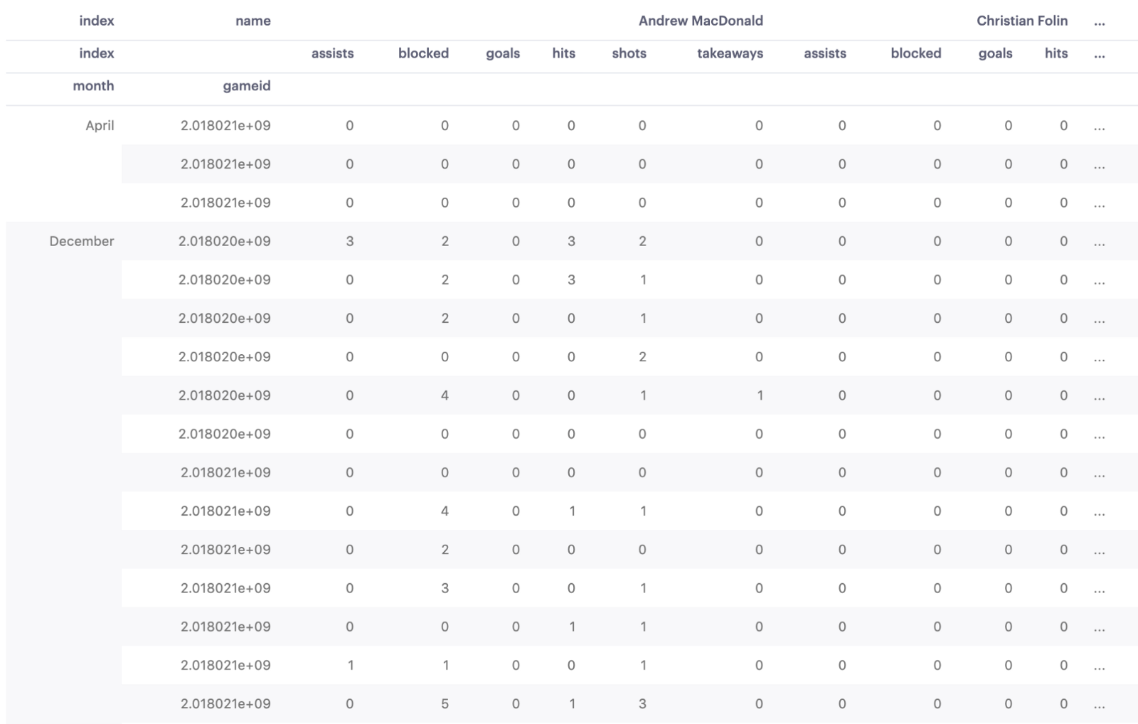
Each of our columns now has two labels! By repeating each stat per player on the team, it's much easier for us to draw conclusions about individual player performance! For instance, let's see what kind of numbers Giroux put up in October:
# Get Claude Giroux's stats for October 2018
girouxDF = pivotDF.loc['October', 'Claude Giroux']
print(girouxDF)
This gives us the cross-section of values where row labels match October and column labels match Giroux:
| Claude Giroux | |||||||
|---|---|---|---|---|---|---|---|
| game_id | assists | blocked | goals | hits | shots | takeaways | |
| October | 2018020014 | 1 | 0 | 0 | 0 | 0 | 0 |
| 2018020026 | 1 | 0 | 0 | 0 | 2 | 0 | |
| 2018020036 | 2 | 0 | 0 | 0 | 4 | 0 | |
| 2018020042 | 1 | 0 | 1 | 0 | 7 | 0 | |
| 2018020058 | 0 | 0 | 0 | 0 | 2 | 0 | |
| 2018020080 | 0 | 0 | 2 | 2 | 8 | 1 | |
| 2018020092 | 2 | 0 | 0 | 0 | 5 | 0 | |
| 2018020102 | 1 | 0 | 0 | 0 | 0 | 1 | |
| 2018020118 | 0 | 0 | 0 | 0 | 5 | 3 | |
| 2018020134 | 0 | 1 | 0 | 1 | 5 | 0 | |
| 2018020149 | 0 | 0 | 0 | 1 | 2 | 0 | |
| 2018020176 | 2 | 0 | 0 | 0 | 4 | 0 |
That's beautiful. The awesome thing about what we've just accomplished is we didn't destroy or modify any data to get to this point. We're still using the same dataset we started with: the only difference is the relationships we've added with indexes.
Finally, let's aggregate these values to give us totals for the month of October, just for kicks:
# Aggregate Giroux's stats
giroux_df = pivot_df.loc['October', 'Claude Giroux'].sum()
print(giroux_df)
Getting a player's stats for a given month
Output:
assists      10
blocked       1
goals         3
hits          4
shots        44
takeaways     5
dtype: int64