
There's a trend among those using Jupyter Notebooks (or equivalent) which leads me to believe humanity is coming to an important realization: Google Maps, as an API is expensive.
Regardless if Google maps is embedded as a consumer-facing widget, or part of a routine data-pipeline, a single surge of high-traffic can leave enterprises with price tags in the hundreds of thousands of dollars. In fact, I can hardly remember a product where this hadn't become the case. One can hardly blame the search engine; after all, our tendency to ignore the Terms and Service agreements (as well as payment policies) has always been core to the Google business model. Even then, there are enough enterprises to go around to turn a blind eye and actually pay such a bill willingly without exploring alternatives.
Data Scientists in particular have no excuse for inaction when it comes to seeking a better alternative. As it turns out, there is one, and it is Cheaper, Easier, and perhaps more Fully Featured than its Google Maps counterpart. That product is Mapbox.
Mapbox is much more than a Google API clone. The web product offers a plethora of UI-driven features that we can use to customize maps as well as save or effortlessly transform raw data into workable GeoJSON data without even touching an API (which, mind you, there is.... with SDKs in every conceivable language). We're going to create a quick map visualization incorporating some real data to get introduced to Mapbox's functionality, but this is only the beginning. Download the line we'll see just how easy it is to incorporate Mapbox in products like Plot.ly Dash or even Jupyter Notebooks.
X Marks the Spot
Before straying from reigning champion Google Maps, it's worth exploring the significance of the metric that brought us here first: price.
Murphy's law clearly states "Cash Rules Everything Around Me, C.R.E.A.M; get the money, Dolla dolla bill y'all." Given this reality, a minimum requirement for Mapbox should be it's pricing model when compared to Google's.
Mapbox Pricing Tiers
| Price | Web apps | Mobile SDKs |
|---|---|---|
|
Free to Start $0 |
50,000 map views /mo 50,000 Geocoding requests /mo 50,000 Directions requests /mo 50,000 Matrix elements /mo 50,000 Tilequery requests /mo |
50,000 map views /mo 50,000 Geocoding requests /mo 50,000 Directions requests /mo 50,000 Matrix elements /mo 50,000 Tilequery requests /mo |
|
Additional Usage $0.50 |
50,000 map views /mo 50,000 Geocoding requests /mo 50,000 Directions requests /mo 50,000 Matrix elements /mo 50,000 Tilequery requests /mo |
50,000 map views /mo 50,000 Geocoding requests /mo 50,000 Directions requests /mo 50,000 Matrix elements /mo 50,000 Tilequery requests /mo |
Compare this to Google's transparent pricing structure:
Google API Pricing Tiers
| Price | Web apps | Mobile SDKs |
|---|---|---|
|
Starter Pack Brown Paper Bag full of $20s |
5 and a half map views /mo 11 times thinking about the API /mo 6 verbal mentions of "Google" /mo 2 directions to shitty parties /mo 8 visits to anywhere /mo |
9 Android unlocks /mo 12 Google queries for restaurants /mo 3 "OK Google" queries /mo 7 Accidental app opens /mo 1 Creating the next "Uber for X" /mo |
|
Additional Usage Eleventy Billion Dollars |
Unlimited Requests!* *See Pricing |
Unlimited Requests!* *See Pricing |
Seems like a convincing point in the win column for Mapbox. If we stay within reason, Mapbox can essentially serve us as an entirely free service.
Surely we must be missing something since we're opting for free services though, right? How do Mapbox visualizations stack up against Google Maps?
Pardon my French here, but hot damn that map is dope. There are plenty more examples where that came from, but it's clear that Mapbox has lowkey stolen the hearts of the scientific analysis market, while Google concerns itself on the consumer and business markets.
Tonight's Itinerary: Creating Dope Maps
To make some data art, we have a few items on our checklist:
- Obtain a dataset with location-based data: In our case of routing, we need a dataset with a set origin and destination per row.
- Create direction object routes by running our dataset through the Mapbox API.
- Create a styled map for our presentation by using Mapbox's style editor.
- Overlay our route data on our beautiful map.
Step 1: Get Some Free Data
Now that we've properly shit-talked Google, let's use Google. We're going to need to get some good data, and BigQuery has some awesome free datasets that we can run wild with. I'll be opting for NYC's dataset on Citibike trips, as it provides a clean set of data where starting and ending coordinates are always present.
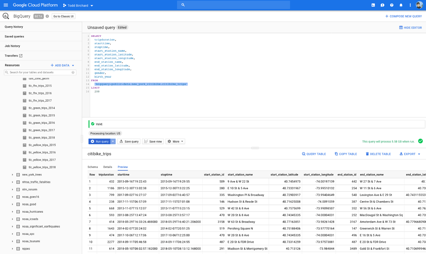
(As a side note, BigQuery is great. Even if you're only somewhat versed in SQL, BigQuery's syntax is essentially whatever your first guess would be.)
Granted we only need the start and end locations to make our map, but i decided to take a bit extra for curiosity's sake:
| start_name | start_latitude | start_longitude | end_name | end_latitude | end_longitude |
|---|---|---|---|---|---|
| 1 Ave & E 15 St | 40.732218530 | -73.981655570 | 1 Ave & E 18 St | 40.733812192 | -73.980544209 |
| 1 Ave & E 30 St | 40.741443870 | -73.975360820 | E 39 St & 2 Ave | 40.747803730 | -73.973441900 |
| 1 Ave & E 62 St | 40.761227400 | -73.960940220 | E 75 St & 3 Ave | 40.771129270 | -73.957722970 |
| 2 Ave & E 99 St | 40.786258600 | -73.945525790 | 3 Ave & E 112 St | 40.795508000 | -73.941606000 |
| 3 St & 3 Ave | 40.675070500 | -73.987752260 | 10 St & 7 Ave | 40.666207800 | -73.981998860 |
| 3 St & Prospect Park West | 40.668132000 | -73.973638310 | 3 St & Prospect Park West | 40.668132000 | -73.973638310 |
| 6 Ave & W 33 St | 40.749012710 | -73.988483950 | W 37 St & 5 Ave | 40.750380090 | -73.983389880 |
| 8 Ave & W 52 St | 40.763707390 | -73.985161500 | Central Park S & 6 Ave | 40.765909360 | -73.976341510 |
| 11 Ave & W 41 St | 40.760300960 | -73.998842220 | W 34 St & 11 Ave | 40.755941590 | -74.002116300 |
| 12 Ave & W 40 St | 40.760875020 | -74.002776680 | W 42 St & 8 Ave | 40.757569900 | -73.990985070 |
| Allen St & E Houston St | 40.722055000 | -73.989111000 | Mott St & Prince St | 40.723179580 | -73.994800120 |
| Allen St & Hester St | 40.716058660 | -73.991907590 | Greenwich St & N Moore St | 40.720434110 | -74.010206090 |
| Amsterdam Ave & W 73 St | 40.779668090 | -73.980930448 | E 85 St & 3 Ave | 40.778012030 | -73.954071490 |
| Bank St & Hudson St | 40.736528890 | -74.006180260 | MacDougal St & Prince St | 40.727102580 | -74.002970880 |
| Bank St & Washington St | 40.736196700 | -74.008592070 | W 4 St & 7 Ave S | 40.734011430 | -74.002938770 |
| Barclay St & Church St | 40.712912240 | -74.010202340 | Clinton St & Tillary St | 40.696192000 | -73.991218000 |
| Berkeley Pl & 7 Ave | 40.675146839 | -73.975232095 | West Drive & Prospect Park West | 40.661063372 | -73.979452550 |
| Bialystoker Pl & Delancey St | 40.716226440 | -73.982612060 | Reade St & Broadway | 40.714504510 | -74.005627890 |
| Broadway & W 24 St | 40.742354300 | -73.989150760 | South End Ave & Liberty St | 40.711512000 | -74.015756000 |
| Broadway & W 29 St | 40.746200900 | -73.988557230 | Stanton St & Chrystie St | 40.722293460 | -73.991475350 |
| Broadway & W 56 St | 40.765265400 | -73.981923380 | Broadway & W 49 St | 40.760683271 | -73.984527290 |
| Broadway & W 58 St | 40.766953170 | -73.981693330 | 5 Ave & E 78 St | 40.776321422 | -73.964273930 |
| Cadman Plaza E & Red Cross Pl | 40.699917550 | -73.989717730 | Leonard St & Church St | 40.717571000 | -74.005549000 |
| Cadman Plaza E & Tillary St | 40.695976830 | -73.990148920 | Lawrence St & Willoughby St | 40.692361780 | -73.986317460 |
| Carmine St & 6 Ave | 40.730385990 | -74.002149880 | W 27 St & 7 Ave | 40.746647000 | -73.993915000 |
| Central Park W & W 96 St | 40.791270000 | -73.964839000 | W 52 St & 6 Ave | 40.761329831 | -73.979820013 |
| Central Park West & W 76 St | 40.778967840 | -73.973747370 | Central Park S & 6 Ave | 40.765909360 | -73.976341510 |
Step 2: Style a Sexy Map in Mapbox Studio
Mapbox provides a superb web UI labeled “studio” interface to help us get started. The “studio” web UI is separated into three parts: custom map styles, tilesets, and datasets.
These three sections can be summarized as:
- Styles: Custom map styles editable via a GUI, which produce a stylesheet for convenience
- Tilesets: Map overlays we can apply from our own data or otherwise to segment geographical areas
- Datasets: Data containing anything from points on a map to complex direction routes we can overlay atop our map.
Here's a quick look at the Map style editor:
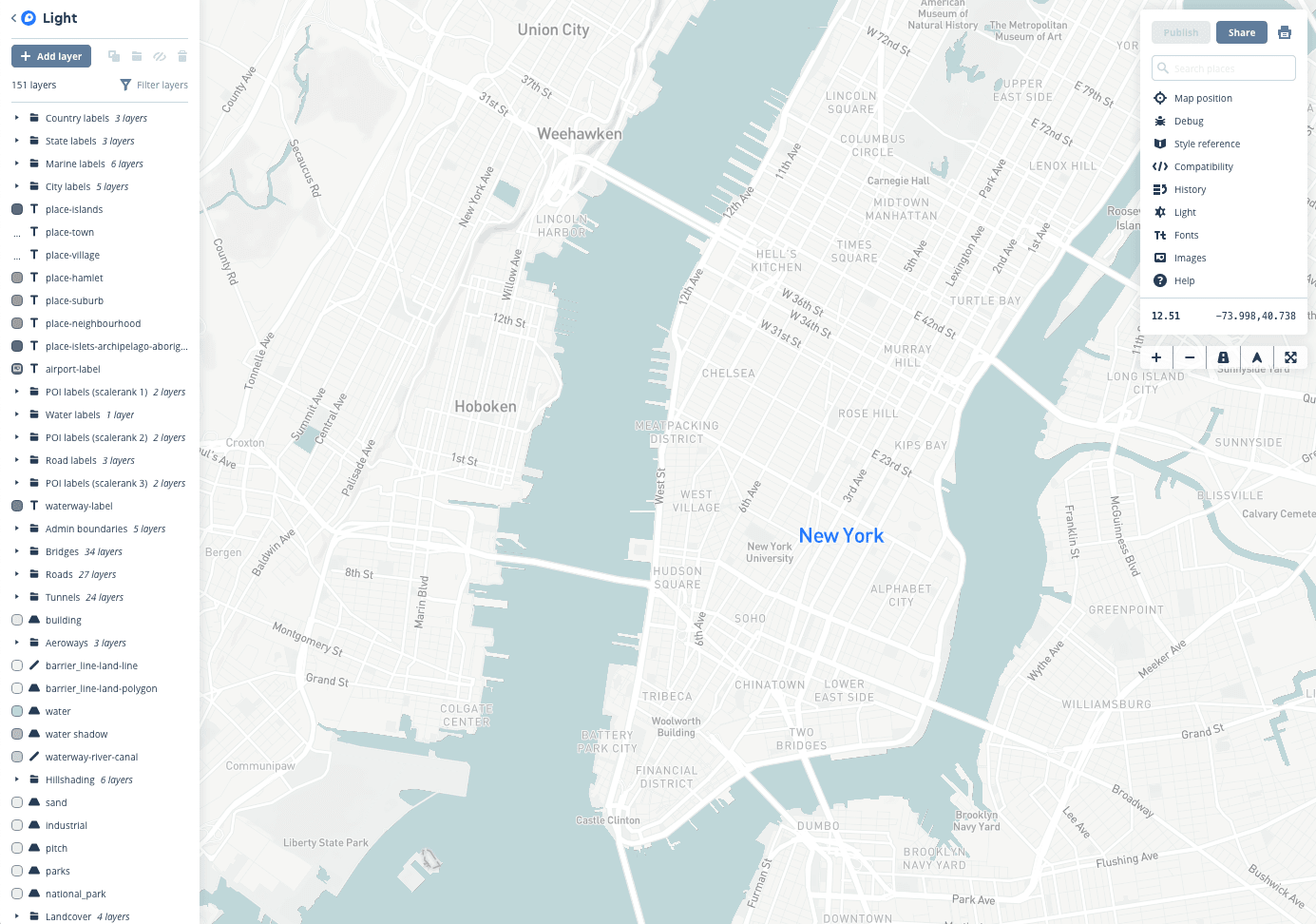
Save your styled map once you find it to be adequately attractive. We'll need it for later.
Step 4: Start a Flask App
Of course we're making a Flask app; is there even any other kind? We'll be using the Flask Application Factory setup as we usually do, so we should end up with a file structure as below. If you feel like you're getting ahead of ourself, checkout our post on structuring Flask applications.
mapbox-app
├── /application
│   └── __init__.py
├── /datasets
│   ├── data.json
│   └── output.csv
├── /maps
│   ├── __init__.py
│   ├── /templates
│   │    └── index.html
│   ├── views.py
│   └── plots.py
├── start.sh
├── settings.py
├── wsgi.py
├── Pipfile
├── README.md
└── requirements.txtTo mix things up a bit we'll use a shell script this time to handle envars and running our script. Start by creating start.sh:
# start.sh

export FLASK_APP=wsgi.py
export FLASK_DEBUG=1
export APP_CONFIG_FILE=settings.py
flask runYes, we'll be using settings.py as our config file for a change. Ahhh, just like the Django days. This file should contain a Mapbox access token. Mapbox provides you with a public token by default in many of its tutorials (noted by the pk prefix for 'public key' - contrast this with sk for 'secret key'). If you'd like to do anything meaningful with Mapbox, you'll have to retrieve a secret key via the UI. Then we can add this token to settings.py as such:
MAPBOX_ACCESS_TOKEN="sk.eyJ1IB&F^&f^R&DFRUYFTRUctyrcTYRUFrtCFTYDYTuEg"Finally, here's a look at application/__init__.py just to make sure we're on the same page:
from flask import Flask

def create_app():
    """Construct the core application."""
    app = Flask(__name__)
    app.config.from_envvar('APP_CONFIG_FILE', silent=True)

    with app.app_context():
        # Construct map blueprint
        from maps import mapviews
        app.register_blueprint(mapviews.map_blueprint)

return appStep 5: Create a Blueprint for Your Map
You may have noticed we registered this Blueprint in the previous step. Create a /maps directory which we'll set as a module; we'll need this to handle the view, model (or just data), and controller (routes.py as seen below).
routes.py
from flask import Blueprint, render_template, request
from flask import current_app as app
from . import locations


map_blueprint = Blueprint(
    'map',
    __name__,
    template_folder='templates',
    static_folder='static'
)
plot_locations = locations.LocationData()


# Landing Page
@map_blueprint.route('/', methods=['GET'])
def map():
    return render_template(
        'index.html',
        ACCESS_KEY=app.MAPBOX_ACCESS_KEY,
        locations=plot_locations.get_plots,
        title="CitiBike Mapbox App."
)templates/index.jinja2
<!DOCTYPE html>
<html>
<head>
  <meta charset='utf-8' />
  <title>{{title}}</title>
  <meta name='viewport' content='initial-scale=1,maximum-scale=1,user-scalable=no' />
  <script src='https://api.tiles.mapbox.com/mapbox-gl-js/v0.49.0/mapbox-gl.js'></script>
  <link href='https://api.tiles.mapbox.com/mapbox-gl-js/v0.49.0/mapbox-gl.css' rel='stylesheet' />
  <style>
    body { margin:0; padding:0; }
    #map { position:absolute; top:0; bottom:0; width:100%; }
  </style>
</head>
<body>

<div id='map'></div>
<script>
mapboxgl.accessToken = {{MAPBOX_ACCESS_TOKEN}};
const map = new mapboxgl.Map({
  container: 'map',
  style: 'mapbox://styles/toddbirchard/cjpij1gfhghiy2spetf5w998w',
  center: [-73.981856, 40.703820],
  zoom: 11.1,

});

map.on('load', function(e) {
  // Add the data to your map as a layer
  map.addLayer({
    id: 'locations',
    type: 'symbol',
    // Add a GeoJSON source containing place coordinates and information.
    source: {
      type: 'geojson',
      data: {{locations}}
    },
    layout: {
      'icon-image': 'restaurant-15',
      'icon-allow-overlap': true,
    }
  });
});
</script>

</body>
</html>data.py
Normally this is where we'd use the magic of the Mapbox API to get coordinates, route objects, or whatever it is your heart hopes to plot. This is intended to be intro post, so let's break that logic out for another time and use a dataset Mapbox would be happy to receive for the sake of results.
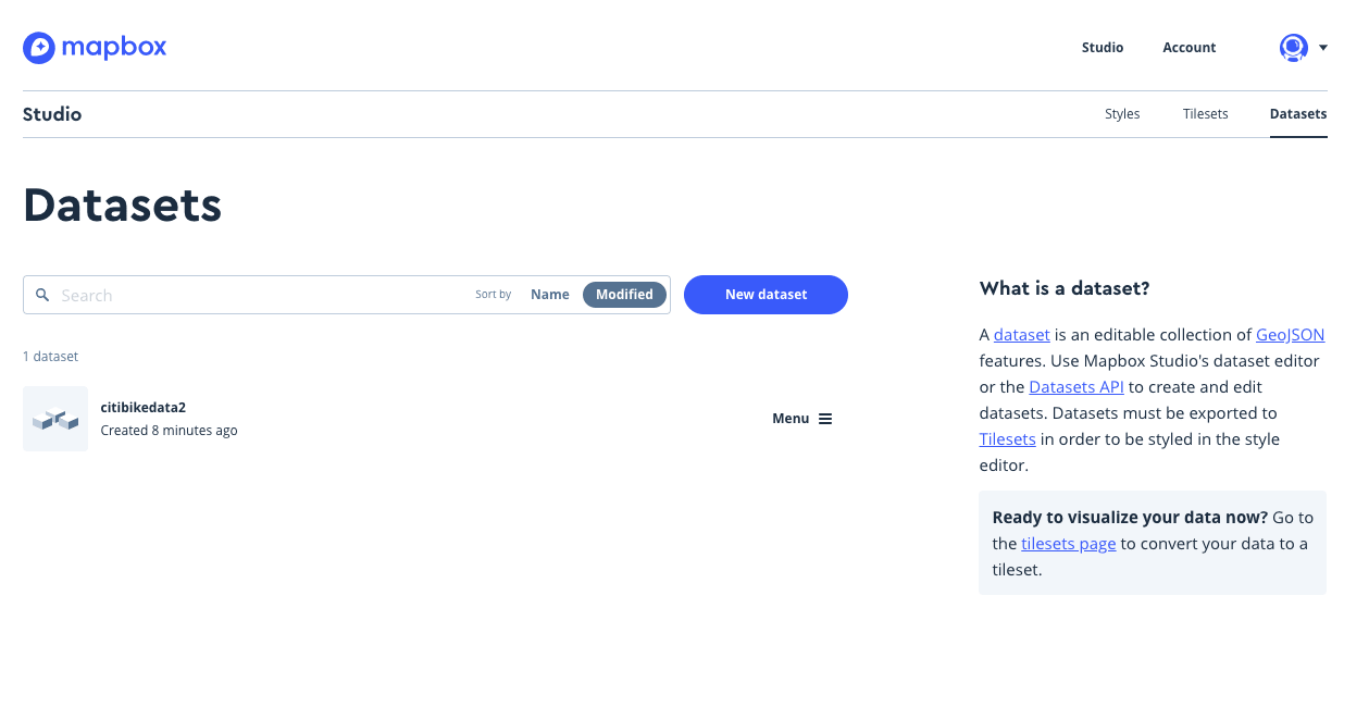
Step 6: Uploading our Dataset via Mapbox Studio
Mapbox graciously lets us upload our data via their Studio UI, which does the unthinkable; immediately upon upload, Mapbox will take the data we give it (whether it be CSV, GeoJSON, etc) and immediately parse it in a way that makes sense. Upload your dataset at https://www.mapbox.com/studio/datasets/:
Next, Mapbox shows us a preview of our data before we even know what happened:
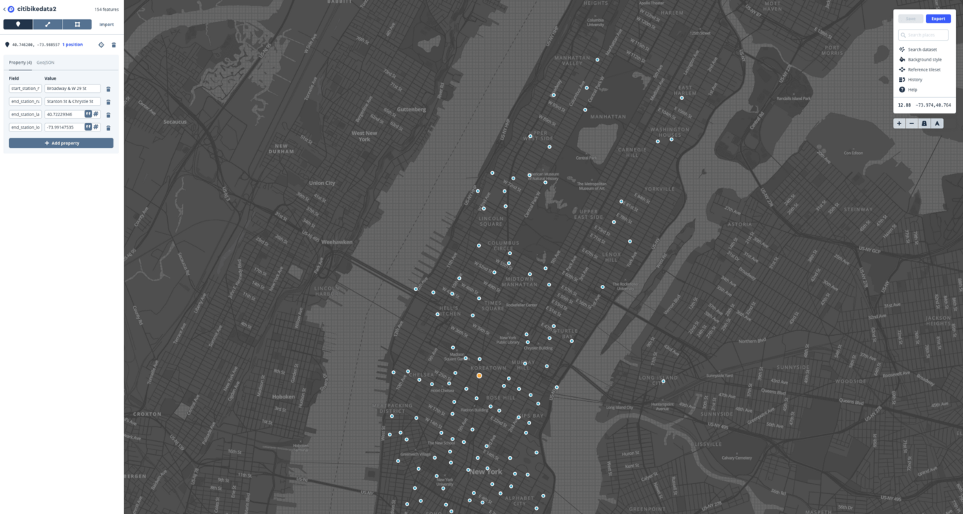
Step 7: Do It in Flask
After uploading your dataset via Mapbox studio, you can actually redownload the data with a subtle twist: your data will be automatically formatted as GeoJSON: the format of JSON objects Mapbox uses to plot points, draw routes, etc.
Since we've had a long day, I'll allow you to download this pre-formatted data and hardcore the values in to your Map view. You're getting off easy for now, but next time we're doing this programmatically ;).
<!DOCTYPE html>
<html>

<head>
  <meta charset='utf-8' />
  <title>{{title}}</title>
  <meta name='viewport' content='initial-scale=1,maximum-scale=1,user-scalable=no' />
  <script src='https://api.tiles.mapbox.com/mapbox-gl-js/v0.49.0/mapbox-gl.js'></script>
  <link href='https://api.tiles.mapbox.com/mapbox-gl-js/v0.49.0/mapbox-gl.css' rel='stylesheet' />
  <style>
    body {
      margin: 0;
      padding: 0;
    }

    #map {
      position: absolute;
      top: 0;
      bottom: 0;
      width: 100%;
    }
  </style>
</head>

<body>

  <div id='map'></div>
  <script>
    mapboxgl.accessToken = '{{ACCESS_KEY}}';
    const map = new mapboxgl.Map({
      container: 'map',
      style: 'mapbox://styles/toddbirchard/cjpij1oxl3hiy2spetf5w998w',
      center: [-73.981856, 40.703820],
      zoom: 11.1,

    });


    map.addLayer({
      "id": "points",
      "type": "symbol",
      "source": {
        "features": [{
            "type": "Feature",
            "properties": {
              "start_station_name": "Central Park West & W 76 St",
              "end_station_name": "Central Park S & 6 Ave",
              "end_station_latitude": "40.76590936",
              "end_station_longitude": "-73.97634151"
            },
            "geometry": {
              "coordinates": [
                -73.973747,
                40.778967
              ],
              "type": "Point"
            },
            "id": "000a1f944d4dd786d9e7ed04620af02b"
          },
          {
            "type": "Feature",
            "properties": {
              "start_station_name": "W 64 St & West End Ave",
              "end_station_name": "W 70 St & Amsterdam Ave",
              "end_station_latitude": "40.77748046",
              "end_station_longitude": "-73.98288594"
            },
            "geometry": {
              "coordinates": [
                -73.987537,
                40.774528
              ],
              "type": "Point"
            },
            "id": "01d8c19524f067a3f4712653265e0a49"
          },
          {
            "type": "Feature",
            "properties": {
              "start_station_name": "E 20 St & FDR Drive",
              "end_station_name": "W 13 St & 7 Ave",
              "end_station_latitude": "40.73781509",
              "end_station_longitude": "-73.99994661"
            },
            "geometry": {
              "coordinates": [
                -73.975738,
                40.733142
              ],
              "type": "Point"
            },
            "id": "038ac5403b136e34874a7278f64d4e95"
          },
          {
              \\ --------------------------------------
              (etc etc....)
               \\ --------------------------------------
          },
          {
            "type": "Feature",
            "properties": {
              "start_station_name": "Mercer St & Bleecker St",
              "end_station_name": "1 Ave & E 30 St",
              "end_station_latitude": "40.74144387",
              "end_station_longitude": "-73.97536082"
            },
            "geometry": {
              "coordinates": [
                -73.996621,
                40.727063
              ],
              "type": "Point"
            },
            "id": "ff1daf9aadbf0cd6b788bd76f0a3f333"
          }
        ],
        "type": "FeatureCollection"
      },
      "layout": {
        "icon-image": "{icon}-15",
        "text-field": "{title}",
        "text-font": ["Open Sans Semibold", "Arial Unicode MS Bold"],
        "text-offset": [0, 0.6],
        "text-anchor": "top"
      }
    });
  </script>

</body>

</html>
Uncharted Territory
There's way more for us to explore in Mapbox. Stay tuned for the rest of this series as we explore generating GeoData programmatically, and build interactive applications to really get users involved in map data by letting them control constraints such as time, etc.