

Something we've only begun to touch on so far is the benefit of utilizing Apache Spark is larger-scale data pipelines. Spark is a quintessential part of the Apache data stack: built on top of Hadoop, Spark is intended to handle resource-intensive jobs such as data streaming and graph processing.
Much of Spark's allure comes from the fact that it is written in Scala & Java. Java and its offshoot languages are notorious for running extremely memory-heavy at run time, which can be used to our advantage. Because our jobs become predictably resource-intensive as everything is stored in memory, this allows us to scale up our Spark Clusters to accommodate accordingly.
A Note About Spark vs. Hadoop
It's crucial for us to understand where Spark fits in the greater Apache ecosystem. Technically, Spark is built atop of Hadoop: Spark borrows a lot from Hadoop's distributed file system, thus comparing "Spark vs. Hadoop" isn't an accurate 1-to-1 comparison. Instead, it's best to think of Spark as being an alternative to Hadoop's MapReduce.
When compared to Hadoop's MapReduce, Spark runs faster. Spark stores DataFrames in memory until otherwise stated, thus giving it a speed bonus over MapReduce, which writes to disk. Of course, Spark comes with the bonus of being accessible via Spark's Python library: PySpark.
If you're interested in learning how these two play together, I recommend this video which breaks this down quite nicely. If you're still a bit green to Hadoop's MapReduce, look no further than this video, which is the best explanation I've found to date.
Using Databricks to Get Started
Spinning up a Spark cluster is a topic that deserves a post in itself - it's a non-trivial process that varies per cloud provider and isn't necessarily the right place to start for those just learning Spark (I also have zero desire to cover this). This is where Databricks comes in.
Databricks is a private company co-founded by the original creator of Apache Spark. Databricks provides a clean notebook interface (similar to Jupyter) which is preconfigured to hook into a Spark cluster. Thus, we can dodge the initial setup associated with creating a cluster ourselves. Databricks' free Community Tier is perhaps the best way for anybody to get started learning Spark.
Navigating the Databricks Interface
If we wanted, we could very well allow Databricks to own our entire Spark stack, aside from maybe where we keep our final data. Check it out the various tabs that make up the Databricks interface:
- Data: This is where we control the input of data. Databricks is heavily integrated with AWS and Azure.
- Clusters: Options for scaling our cluster of servers. Any changes made here are directly reflected in AWS.
- Jobs: The cool things about Databricks notebooks is that they don't have to be just notebooks. By linking our notebooks to scheduled jobs, we can use our notebooks as actual scripts to execute regularly. Thus, our notebooks become entirely functional production code as a result.
- Import Library: This one is a bit hard to find… it lives under Databricks > Import library. This is the tool we use to import third-party Python (or Java) libraries for usage in our notebooks. The easiest way to accomplish this is by selecting “PyPI”, and then provide the name of the library (ie: pandas). This will install the library on your cluster and make it available for use.
Uploading Sample Data
The easiest way to add some data to work with in Databricks is via their UI. Going back to the data tab, we have the options to hook into an S3 bucket, upload a CSV, or even select from sources such as Amazon Redshift or Apache Kaftka. Unfortunately, Google Cloud is not yet supported by Databricks 😡.
We'll keep things simple and upload a CSV to kick things off:

Upon uploading, we immediately get the option to Create Table in Notebook. It's best to move forward with this option, as it shows us how to programmatically load data into Spark for the future. Selecting this option will create a new notebook with some boilerplate for us.
Types of Structured Data in Spark
Before we load up our data, we should be aware of the different types of data we can work with in Spark. Spark started off with a single data structure called RDDs, and has expanded into two-dimensional data by adding DataFrames and Datasets:
- An RDD is a set of data populated across our many Spark clusters, hence their name (Resilient Distributed Datasets). RDD data is stored as either a list or a key/value store. RDDs serve many purposes, such as parsing text files into workable data types which can then be repurposed into DataFrames.
- DataFrames are an evolution of RDDs designed to be easier to use, similar to how we might expect SQL tables to work. As a result, DataFrames created from structured data only. Unlike RDDs, DataFrames automatically have a number of optimizations applied to them which make working with structured data faster and easier. Unlike RDDs, however, DataFrames cannot be modified after their initial creation.
- Datasets are a form of tabular data limited to Scala (booo). Datasets are similar to DataFrames, but add an additional layer of type safety to disallow data of the wrong type to fall into the wrong columns.
DataFrames and Datasets together make up the part of Spark frequently referred to as "Spark SQL," which isn't to be confused with SQL functions we can execute in Spark. Truthfully there are a lot of naming conventions that leave a lot to be desired in Spark.
Anatomy of a Spark DataFrame
RDDs may have been the original way to work with data in Spark, but these days DataFrames are the bread and butter. This isn't to downplay the importance of RDDs - DataFrames are built on the same logic as RDDs, and we absolutely must know the ins-and-outs of RDDs if we want to consider ourselves respectable Spark users. That said, if you're looking to get pick up as much as possible about Spark in a short period of time, DataFrames are what we should focus on.
There are three properties of DataFrames we should be aware of:
- Immutable: Spark DataFrames like to be created once upfront, without being modified after the fact.
- Distributed: Spark DataFrames are fault-tolerant and highly-available, much like vanilla Hadoop. Thus, we are at little risk of something going horribly wrong and wiping our DataFrame from existence due to external factors - if a node in our Spark cluster goes down, Spark can charge forward regardless.
- Lazy evaluation: DataFrame tasks are not executed until explicitly executed. This shouldn't be a new concept; those familiar with the PEP style guide know that most data-related tasks in Python are executed this way.
Great, but what does working with a Spark DataFrame look like? The general structure of modifying a Spark DataFrame typically looks like this:
new_df = original_df. \
    transformation_1(original_df). \
    transformation_2(original_df). \
transformation_3(original_df)As we mentioned before, Spark DataFrames are immutable, so we need to create a new DataFrame from our original each time we'd like to make adjustments (AKA: new_df = original_df.etc()).
From there, we can chain together transformations to ensure we don't create a new DataFrame per transformation, which would be a waste of memory.
Creating Spark DataFrames
We can create Spark DataFrames from a number of different sources such as CSVs, JSON files, or even by stitching together RDDs. We've already uploaded a CSV, so we'll start there.
Creating DataFrames from CSVs
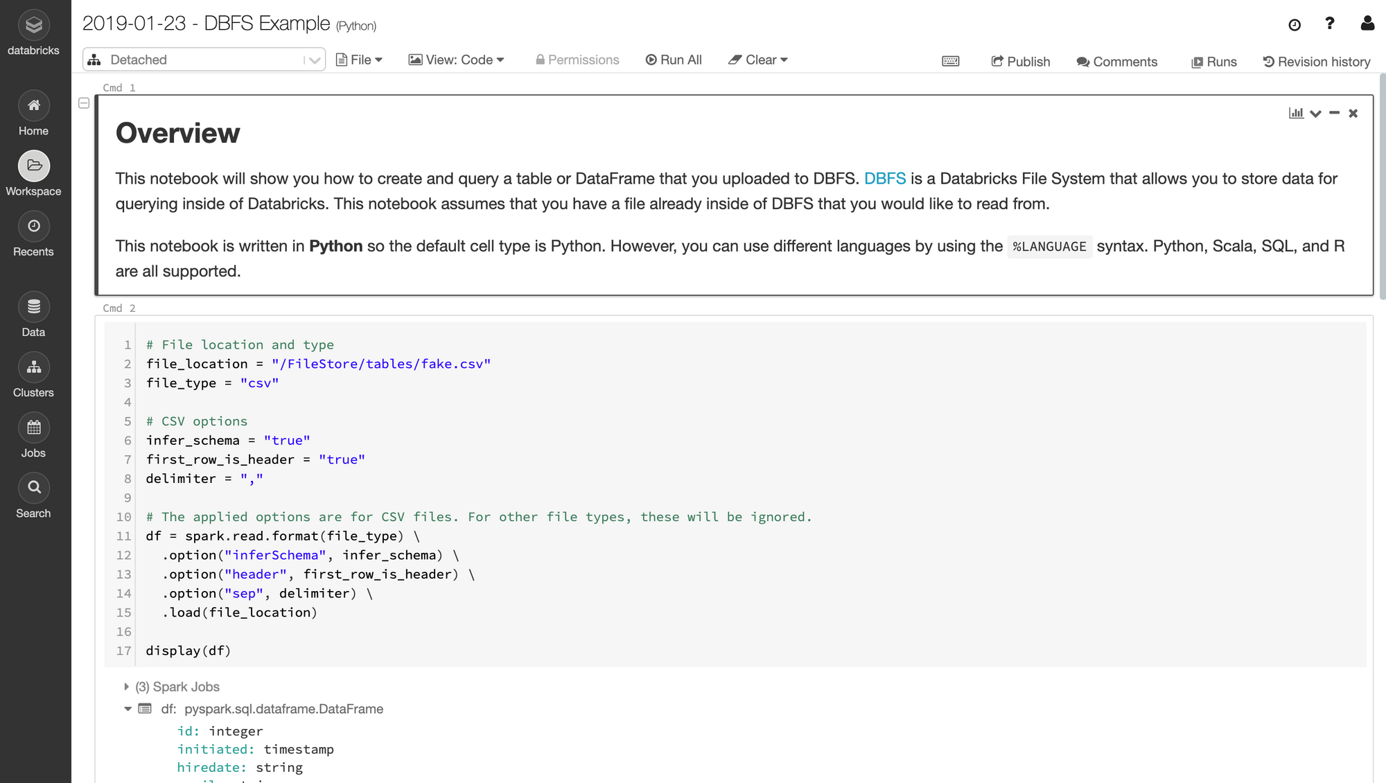
If you selected the Create Table in Notebook option when you uploaded your CSV, you should see a notebook with a first cell that looks like this:
# File location and type
FILE_LOCATION = "/FileStore/tables/posts.csv"
FILE_TYPE = "csv"

# CSV options
INFER_SCHEMA = "false"
FIRST_ROW_IS_HEADER = "false"
DELIMITER = ","

# The applied options are for CSV files.
df = spark.read.format(FILE_TYPE) \
  .option("inferSchema", INFER_SCHEMA) \
  .option("header", FIRST_ROW_IS_HEADER) \
  .option("sep", DELIMITER) \
  .load(FILE_LOCATION)

display(df)This cell is showing us the preferred method for creating a DataFrame from a CSV file. The first thing that happens is spark.read.format("csv"): this is telling Spark that we're about to read data (yes, we can write this way also....hang in there). We tell Spark that the file we'll be passing will be a CSV by using .format(). We could also specify text, JSON, etc.
Notice how we have a few option()s chained to this read? Each "option" is specifying configuration which determine how our CSV should be created :
infer_schema: Analyzes patterns in the data we've uploaded to automatically downcast each column to the proper data type. Assuming your data is coherent, I've found this feature to be surprisingly accurate. Let's leverage this functionality by setting the value to "true".first_row_is_header: When true, treats the first row of our CSV as our DataFrame's column names.delimiter: The character used to signal the end of a column (defaults to a comma as is the case with CSVs). We can leave this as",", unless your "Comma Separated Values" are separated by something other than commas... you madman.
If you're like me, you might already be thrown off by some of the weird syntax things happening here:
- Boolean values in PySpark are sometimes set by strings (either
"true"or"false", as opposed to Python'sTrueorFalse). One might assume that PySpark consistently prefers strings over booleans, but keyword arguments in PySpark expect to be passedTrueandFalse. This is one of many unsavory choices made in the design of PySpark. - You'll recognize "df" as shorthand for DataFrame, but let's not get carried away - working with PySpark DataFrames is much different from working with Pandas DataFrames in practice, even though they're conceptually similar. The syntax and underlying tech are quite different between the two.
- Databricks provides us with a super neat
display()function, which is a much more powerful way of previewing our DataFrames thanprint(). I'll be sure to point out some of the advantages ofdisplay()as we go along.
Our first cell is now ready to rock. Let's see what running this does:
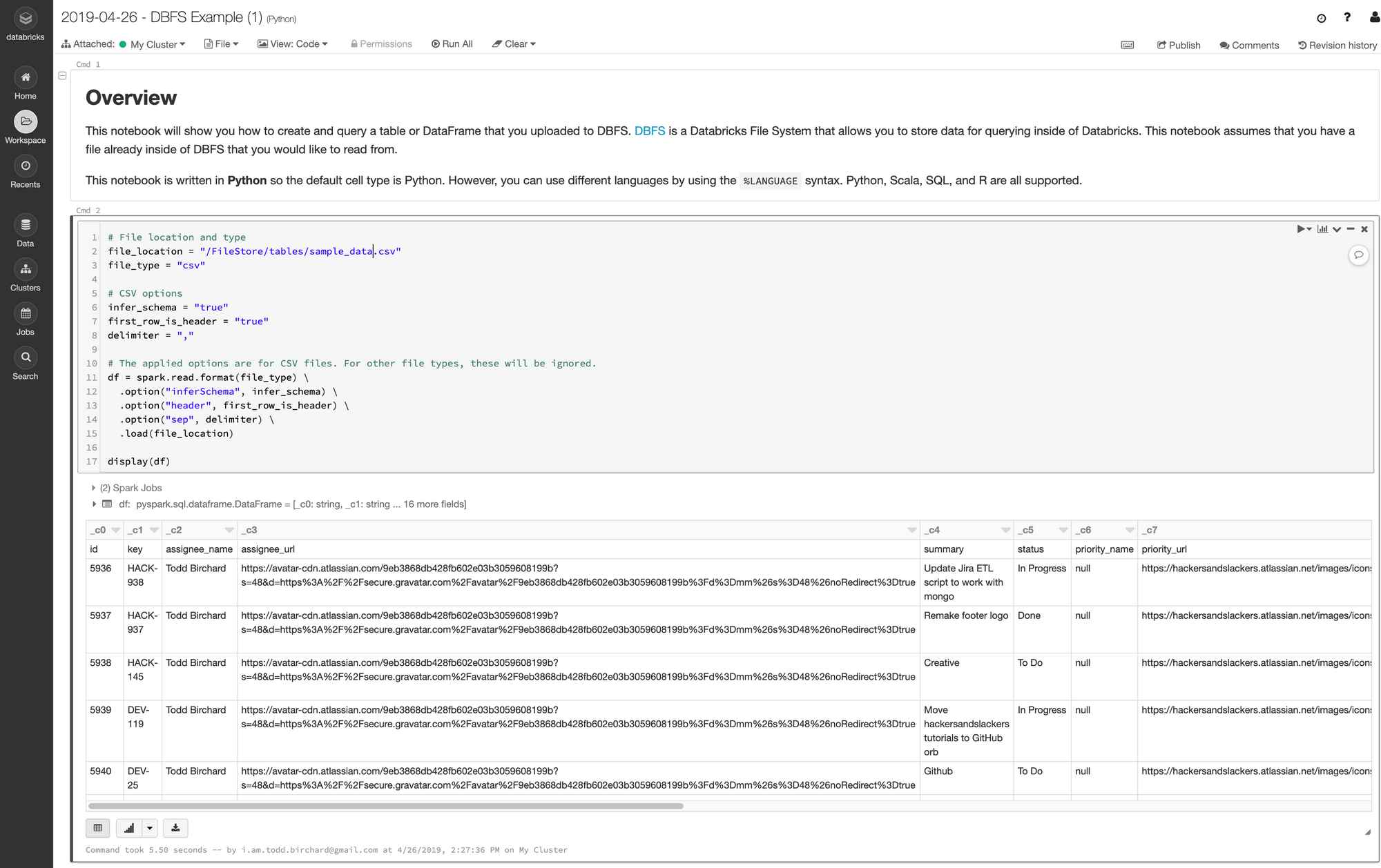
Our data is now loaded into memory!
Creating DataFrames from JSON
Spark also has a built-in method for reading JSON files into DataFrames. Here's the JSON I'll be loading:
[{
    "id": 1,
    "player_name": "Nick Young",
    "team_name": "Lakers"
  },
  {
    "id": 2,
    "player_name": "Lou Williams",
    "team_name": "Lakers"
  },
  {
    "id": 13,
    "player_name": "Lebron James",
    "team_name": "Cavaliers"
  },
  {
    "id": 4,
    "player_name": "Kyrie Irving",
    "team_name": "Cavaliers"
}]Creating a DataFrame from this JSON file is quite simple:
df = spark.read.json(
    "/FileStore/tables/nbaplayers.json",
    multiLine=True
)

display(df)Because our JSON object spans across multiple lines, we need to pass the multiLine keyword argument. Take note of the capitalization in "multiLine"- yes it matters, and yes it is very annoying.
Here's how our data came out:
| id | player_name | team_name |
|---|---|---|
| 1 | Nick Young | Lakers |
| 2 | Lou Williams | Lakers |
| 13 | Lebron James | Cavaliers |
| 4 | Kyrie Irving | Cavaliers |
| 5 | Chris Paul | Lakers |
| 6 | Blake Griffin | Lakers |
| 20 | Kevin Durant | Warriors |
| 17 | Stephen Curry | Warriors |
| 9 | Dwight Howard | Lakers |
| 10 | Kyle Korver | Lakers |
| 11 | Kyle Lowry | Cavaliers |
| 12 | DeMar DeRozan | Cavaliers |
Creating DataFrames From Nested JSON
Quite often we'll need to deal with JSON structured with nested values, like so:
{
  "data": [
    [1, "Nick Young", "Lakers"],
    [2, "Lou Williams", "Lakers"],
    [13, "Lebron James", "Cavaliers"],
    [4, "Kyrie Irving", "Cavaliers"],
    [5, "Chris Paul", "Lakers"],
    [6, "Blake Griffin", "Lakers"],
    [20, "Kevin Durant", "Warriors"],
    [17, "Stephen Curry", "Warriors"],
    [9, "Dwight Howard", "Lakers"],
    [10, "Kyle Korver", "Lakers"],
    [11, "Kyle Lowry", "Cavaliers"],
    [2, "DeMar DeRozan", "Cavaliers"]
  ]
}
Creating a table of this as-is doesn't give much of anything useful; we only get a single column:
| data |
|---|
| [["1","Nick Young","Lakers"],["2","Lou Williams","Lakers"],["13","Lebron James","Cavaliers"],["4","Kyrie Irving","Cavaliers"],["5","Chris Paul","Lakers"],["6","Blake Griffin","Lakers"],["20","Kevin Durant","Warriors"],["17","Stephen Curry","Warriors"],["9","Dwight Howard","Lakers"],["10","Kyle Korver","Lakers"],["11","Kyle Lowry","Cavaliers"],["2","DeMar DeRozan","Cavaliers"]] |
The first step we can take here is using Spark's explode() function. explode() splits multiple entries in a column into multiple rows:
from pyspark.sql.functions import explode


exploded_df = df.select(explode("data").alias("d"))
display(exploded_df).explode() on columns containing multiple values will create a column per valueThe raw data we provided in our nested JSON example was structured in an intentionally vague manner: a single JSON key, containing a list of lists. The intent on how this should translate to tabular data is difficult to interpret even for a human being. When parsing JSON to Dataframes, keys are typically associated with columns, while values populate the aforementioned columns. This data would be interpreted as a single column with a single value.
Spark (and its predecessors) have been in the game a long time, hence methods to handle highly-specific scenarios, such as explode(). explode() accepts one or more column names to "explode," which will create an individual row per iterable value within said column(s).
(We added alias() to this column as well, which modifies the column names after explode() has been executed.)
| d |
|---|
| ["1","Nick Young","Lakers"] |
| ["2","Lou Williams","Lakers"] |
| ["13","Lebron James","Cavaliers"] |
| ["4","Kyrie Irving","Cavaliers"] |
| ["5","Chris Paul","Lakers"] |
| ["6","Blake Griffin","Lakers"] |
| ["20","Kevin Durant","Warriors"] |
| ["17","Stephen Curry","Warriors"] |
| ["9","Dwight Howard","Lakers"] |
| ["10","Kyle Korver","Lakers"] |
| ["11","Kyle Lowry","Cavaliers"] |
| ["2","DeMar DeRozan","Cavaliers"] |
Before we called explode(), our DataFrame was 1 column wide and 1 row tall. Now we have new rows: one per item that lived in our old data column:
This only gets us halfway there- we still need to deal with the fact that we only have 1 column for three values. Since our column is an array, we can access each item fairly easily by getting the value at each index:
new_players_df = exploded_df.select(
    exploded_df.d[0],
    exploded_df.d[1],
    exploded_df.d[2]
)
new_players_df = exploded_df.selectExpr(
    "d[0] as id",
    "d[1] as name",
    "d[2] as team"
)

display(new_players_df)Now we're looking two-dimentionsal:
| id | name | team |
|---|---|---|
| 1 | Nick Young | Lakers |
| 2 | Lou Williams | Lakers |
| 13 | Lebron James | Cavaliers |
| 4 | Kyrie Irving | Cavaliers |
| 5 | Chris Paul | Lakers |
| 6 | Blake Griffin | Lakers |
| 20 | Kevin Durant | Warriors |
| 17 | Stephen Curry | Warriors |
| 9 | Dwight Howard | Lakers |
| 10 | Kyle Korver | Lakers |
| 11 | Kyle Lowry | Cavaliers |
| 2 | DeMar DeRozan | Cavaliers |
Creating DataFrames from RDDs
We're going to save the finer details RDDs for another post, but it's worth knowing that DataFrames can be constructed using RDDs. This is particularly useful when we parse data from unstructured formats and want to work with said data in a tabular format.
To create a DataFrame from an RDD, we use a function called createDataFrame() which we call on the Spark context:
df = sqlContext.createDataFrame(records, schema)

display(df)Records would be our RDD in this case, and schema would be a schema of headers and data types to structure our table. You don't need to know what this means just yet - I'm just trying to spice up this series by adding some dramatic foreshadowing.
Saving Our Data
While most of the work we do will revolve around modifying data in memory, we'll eventually want to save our data to disk at some point. Databricks allows us to save our tables by either creating a temporary table or a persistent table.
Temporary Tables
Creating a "temporary table" saves the contents of a DataFrame to a SQL-like table. These tables are "temporary" because they're only accessible to the current notebook. Temporary tables aren't actually accessible across our cluster by other resources; they're more of a convenient way to say "hold my beer," where your beer is actually data.
We can create temporary tables from any DataFrame by calling either createTempable() or createOrReplaceTempView() on a DataFrame:
# Create a temporary view/table

df.createOrReplaceTempView("my_temp_table")  # Always writes table
df.createTempView("my_temp_table") # Errors out if table existsWe can also accomplish this by calling registerTempTable() on our Spark content:
sc.registerTempTable(df, "my_temp_table")Persistent Tables
Databricks saves tabular data to a Hive metastore, which it manages for you. To write a DataFrame to a table, we first need to call write on said DataFrame. From there we can can saveAsTable():
# Create a permanent table

df.write.saveAsTable('my_permanent_table')
If we want to save our table as an actual physical file, we can do that also:
df.write.format("parquet").saveAsTable("my_permanent_table")Writing SQL in Databricks
You may have noticed that the auto-generated notebook contains a cell which begins with %sql, and then contains some SQL code. % denotes a magic function. In this case, it's a magic function that sets the programming language the cell will be written in. Cells which begin with %sql will be run as SQL code. We created a "Python" notebook thus %python is the default, but %scala, %java, and %r are supported as well.
Writing SQL in a Databricks notebook has some very cool features. For example, check out what happens when we run a SQL query containing aggregate functions as per this example in the SQL quickstart notebook:

We could easily spend all day getting into the subtleties of Databricks SQL, but that's a post for another time.
Welcome To Your New Life
If you're a data engineering in any capacity, you're going to spend a lot of time in Spark. Working with Spark isn't like working in your typical Python data science environment. In fact, there are a lot ways in which working with PySpark doesn't feel like working in Python at all: it becomes painfully obvious at times that PySpark is an API which translates into Scala. As a result, a lot of the dynamic wizard-like properties of Python aren't always at our disposable.
There are a lot of things I'd change about PySpark if I could. That said, if you take one thing from this post let it be this: using PySpark feels different because it was never intended for willy-nilly data analysis. Spark is a big, expensive cannon that we data engineers wield to destroy anything in our paths. If carrying cannons around were easy, then Rambo wouldn't be so badass. If you ever find yourself frustrated with PySpark, remember that you are Rambo.
We've covered a lot here, and yet almost nothing at all (all we've done so far is load data!). If you need some help having any of this sink in, I'd highly suggest creating a free Databricks account and messing around. If not, no big deal... I'm not getting paid for these kind words anyway.