We've had quite a journey exploring the magical world of PySpark together. After covering DataFrame transformations, structured streams, and RDDs, there are only so many things left to cross off the list before we've gone too deep.
To round things up for this series, we're a to take a look back at some powerful DataFrame operations we missed. In particular, we'll be focusing on operations that modify DataFrames as a whole, such as
Joining DataFrames in PySpark
I'm going to assume you're already familiar with the concept of SQL-like joins. To demonstrate these in PySpark, I'll create two simple DataFrames: a customers DataFrame and an orders DataFrame:
# DataFrame 1
valuesA = [
    (1, 'bob', 3462543658686),
    (2, 'rob', 9087567565439),
    (3, 'tim', 5436586999467),
    (4, 'tom', 8349756853250)
]

customersDF = spark.createDataFrame(
    valuesA,
    ['id', 'name', 'credit_card_number']
)

# DataFrame 2
valuesB = [
    (1, 'ketchup', 'bob', 1.20),
    (2, 'rutabaga', 'bob', 3.35),
    (3, 'fake vegan meat', 'rob', 13.99),
    (4, 'cheesey poofs', 'tim', 3.99),
    (5, 'ice cream', 'tim', 4.95),
    (6, 'protein powder', 'tom', 49.95)
]
ordersDF = spark.createDataFrame(
    valuesB,
    ['id', 'product_name', 'customer', 'price']
)

# Show tables
customersDF.show()
ordersDF.show()
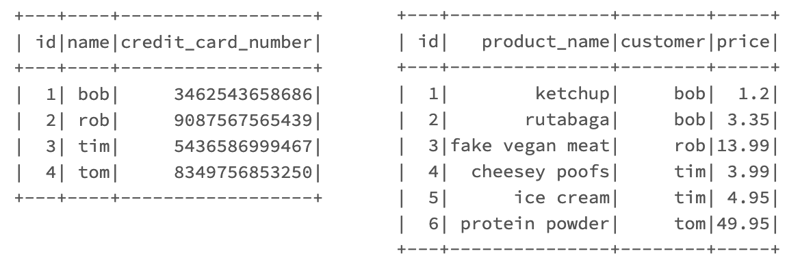
Here's how they look:

Now we have two cliche tables to work with.
Before we join these two tables it's important to realize that table joins in Spark are relatively "expensive" operations, which is to say that they utilize a fair amount of time and system resources.
Inner Joins
Without specifying the type of join we'd like to execute, PySpark will default to an inner join. Joins are possible by calling the join() method on a DataFrame:
joinedDF = customersDF.join(ordersDF, customersDF.name == ordersDF.customer)The first argument join() accepts is the "right" DataFrame that we'll be joining on to the DataFrame we're calling the function on.
Next, we specify the "on" of our join. In our example, we're telling our join to compare the "name" column of customersDF to the "customer" column of ordersDF. Here's how it turned out:
| id | name | credit_card_number | id | product_name | customer | price |
|---|---|---|---|---|---|---|
| 2 | rob | 9087567565439 | 3 | fake vegan meat | rob | 13.99 |
| 3 | tim | 5436586999467 | 4 | cheesey poofs | tim | 3.99 |
| 3 | tim | 5436586999467 | 5 | ice cream | tim | 4.95 |
| 4 | tom | 8349756853250 | 6 | protein powder | tom | 49.95 |
| 1 | bob | 3462543658686 | 1 | ketchup | bob | 1.2 |
| 1 | bob | 3462543658686 | 2 | rutabaga | bob | 3.35 |
Right, Left, and Outer Joins
We can pass the keyword argument "how" into join(), which specifies the type of join we'd like to execute. how accepts inner, outer, left, and right, as you might imagine. how also accepts a few redundant types like leftOuter (same as left).
Cross Joins
The last type of join we can execute is a cross join, also known as a cartesian join. Cross joins are a bit different from the other types of joins, thus cross joins get their very own DataFrame method:
joinedDF = customersDF.crossJoin(ordersDF)Cross joins create a new row in DataFrame #1 per record in DataFrame #2:

Aggregating Data
Spark allows us to perform powerful aggregate functions on our data, similar to what you're probably already used to in either SQL or Pandas. The data I'll be aggregating is a dataset of NYC motor vehicle collisions because I'm a sad and twisted human being:
| borough | contributing_factor_vehicle_1 | contributing_factor_vehicle_2 | cross_street_name | timestamp | latitude | longitude | location | number_of_cyclist_injured | number_of_cyclist_killed | number_of_motorist_injured | number_of_motorist_killed | number_of_pedestrians_injured | number_of_pedestrians_killed | number_of_persons_injured | number_of_persons_killed | off_street_name | on_street_name | unique_key | vehicle_type_code1 | vehicle_type_code2 | zip_code |
|---|---|---|---|---|---|---|---|---|---|---|---|---|---|---|---|---|---|---|---|---|---|
| MANHATTAN | Following Too Closely | Unspecified | LEXINGTON AVENUE | 2019-06-18T12:15:00 | 40.772373 | -73.96079 | (40.772373, -73.96079) | 0 | 0 | 0 | 0 | 0 | 0 | 0 | 0 | EAST 75 STREET | 4154304 | Station Wagon/Sport Utility Vehicle | Box Truck | 10021 | |
| MANHATTAN | Driver Inattention/Distraction | Unspecified | PARK AVENUE | 2019-06-14T13:43:00 | 40.8076 | -73.93719 | (40.8076, -73.93719) | 1 | 0 | 0 | 0 | 0 | 0 | 1 | 0 | EAST 129 STREET | 4152035 | Van | Bike | 10035 | |
| MANHATTAN | Backing Unsafely | Following Too Closely | WEST 158 STREET | 2019-06-11T12:40:00 | 40.83468 | -73.944435 | (40.83468, -73.944435) | 0 | 0 | 0 | 0 | 0 | 0 | 0 | 0 | BROADWAY | 4150129 | Station Wagon/Sport Utility Vehicle | Tractor Truck Diesel | 10032 | |
| BROOKLYN | Driver Inattention/Distraction | Unspecified | 2019-06-11T17:00:00 | 40.72065 | -73.96079 | (40.72065, -73.96079) | 0 | 0 | 0 | 0 | 0 | 0 | 0 | 0 | 58 NORTH 8 STREET | 4150450 | Sedan | Pick-up Truck | 11249 | ||
| MANHATTAN | Unspecified | Unspecified | PARK AVENUE | 2019-06-07T15:30:00 | 40.805058 | -73.93904 | (40.805058, -73.93904) | 0 | 0 | 0 | 0 | 0 | 0 | 0 | 0 | EAST 125 STREET | 4147239 | Bus | Pick-up Truck | 10035 | |
| QUEENS | Traffic Control Disregarded | Failure to Yield Right-of-Way | 58 AVENUE | 2019-06-06T18:40:00 | 40.74554 | -73.7768 | (40.74554, -73.7768) | 0 | 0 | 0 | 0 | 0 | 0 | 0 | 0 | FRANCIS LEWIS BOULEVARD | 4146404 | Sedan | Pick-up Truck | 11364 | |
| QUEENS | Driver Inattention/Distraction | Unspecified | 2019-06-04T15:00:00 | 40.76257 | -73.88856 | (40.76257, -73.88856) | 0 | 0 | 0 | 0 | 0 | 0 | 0 | 0 | 25-38 80 STREET | 4144994 | Station Wagon/Sport Utility Vehicle | Box Truck | 11370 | ||
| BROOKLYN | Failure to Yield Right-of-Way | Unspecified | WEST 20 STREET | 2019-05-31T15:30:00 | 40.5787 | -73.98734 | (40.5787, -73.98734) | 0 | 0 | 0 | 0 | 0 | 0 | 0 | 0 | NEPTUNE AVENUE | 4143848 | Sedan | Flat Bed | 11224 | |
| MANHATTAN | Driver Inattention/Distraction | Unspecified | 2019-05-30T15:00:00 | 40.793224 | -73.97096 | (40.793224, -73.97096) | 0 | 0 | 0 | 0 | 0 | 0 | 0 | 0 | 715 AMSTERDAM AVENUE | 4142113 | Bus | Bus | 10025 |
We're going to become familiar with two functions here: agg() and groupBy(). These are typically used in tandem, but agg() can be used on a dataset without groupBy():
df.agg({"*": "count"}).show()Aggregating without performing groupBy() typically isn't entirely useful:
+--------+
|count(1)|
+--------+
|  1000  |
+--------+Let's derive some deeper meaning from our data by combining agg() with groupby().
Using groupBy()
Let's see which boroughs lead the way in terms of the number of accidents:
import pyspark.sql.functions as f


df
  .groupby('borough')
  .agg(f.count('borough')
  .alias('count'))
  .show()
The results:
+-------------+-----+
| borough     |count|
+-------------+-----+
| QUEENS      | 241 |
| BROOKLYN    | 182 |
| BRONX       | 261 |
| MANHATTAN   | 272 |
|STATEN ISLAND|  44 |
+-------------+-----+Queens leads the way with 241 accidents from our sample size! Get your shit together, Queens. Let's see which borough is the deadliest:
df
  .groupby('borough')
  .agg(f.sum('number_of_persons_injured')
  .alias('injuries'))
  .orderBy('injuries', ascending=False)
  .show()
Here we go:
+-------------+--------+
| borough     |injuries|
+-------------+--------+
| MANHATTAN   |     62 |
| QUEENS      |     59 |
| BRONX       |     57 |
| BROOKLYN    |     47 |
|STATEN ISLAND|     14 |
+-------------+--------+Well... alright then.
Grouping By Multiple Columns
Often times we'll want to group by multiple columns to see more complex breakdowns. Here we group by both borough and "main contributing factor":
aggDF = df
  .groupby('borough', 'contributing_factor_vehicle_1')
  .agg(f.sum('number_of_persons_injured')
  .alias('injuries'))
  .orderBy('borough', 'injuries', ascending=False)

aggDF = aggDF.filter(aggDF.injuries > 1)

display(aggDF)
This will show us the most common type of accidents per borough:
| borough | contributing_factor_vehicle_1 | injuries |
|---|---|---|
| STATEN ISLAND | Driver Inattention/Distraction | 4 |
| STATEN ISLAND | Unspecified | 4 |
| STATEN ISLAND | Failure to Yield Right-of-Way | 3 |
| QUEENS | Driver Inattention/Distraction | 21 |
| QUEENS | Failure to Yield Right-of-Way | 10 |
| QUEENS | Unspecified | 8 |
| QUEENS | Traffic Control Disregarded | 5 |
| MANHATTAN | Driver Inattention/Distraction | 19 |
| MANHATTAN | Unspecified | 17 |
| MANHATTAN | Pedestrian/Bicyclist/Other Pedestrian Error/Confusion | 5 |
| MANHATTAN | Failure to Yield Right-of-Way | 4 |
| MANHATTAN | Passing or Lane Usage Improper | 3 |
| BROOKLYN | Driver Inattention/Distraction | 15 |
| BROOKLYN | Failure to Yield Right-of-Way | 6 |
| BROOKLYN | Unspecified | 5 |
| BROOKLYN | Oversized Vehicle | 4 |
| BROOKLYN | Driver Inexperience | 3 |
| BRONX | Unspecified | 16 |
| BRONX | Driver Inattention/Distraction | 6 |
| BRONX | Driver Inexperience | 6 |
| BRONX | Unsafe Lane Changing | 3 |
| BRONX | Pedestrian/Bicyclist/Other Pedestrian Error/Confusion | 3 |
| BRONX | Passing or Lane Usage Improper | 3 |
| BRONX | Traffic Control Disregarded | 3 |
| BRONX | Failure to Yield Right-of-Way | 3 |
So far we've aggregated by using the count and sum functions. As you might imagine, we could also aggregate by using the min, max, and avg functions. There's one additional function worth special mention as well called corr().
Determining Column Correlation
If you're the scientific type, you're going to love aggregating using corr(). corr() determines whether two columns have any correlation between them and outputs an integer which represent the correlation:
df.agg(corr("a", "b").alias('correlation')).collect()Example output:
[Row(correlation=1.0)]Databricks Visualizations on Aggregations
If you're following along in a Databricks notebook, a ton of cool visualizations come standard with the display() command to complement any aggregations we perform. These are especially useful when trying to understand the distribution of aggregate functions we perform.
I went ahead and pieced together a breakdown of people injured in accidents below. We're splitting our results by borough, and then seeing the distribution of people injured between cyclists and motorists:

While customizing a bar plot, "keys" determines the values across the x-axis.I'm measuring by a number of "values" here, which is to say that multiple measurements across the y-axis will be shown.
This particular chart lends itself well to a stacked bar chart, which we create by specifying bar chart as our display type, and then specifying stacked in the additional options. Databricks allows for all sorts of additional cool visualizations like geographical charts, scatter plots, and way more.
Happy Trails
We've been through a lot on this PySpark journey together. As much as I'd love to keep you here forever, every good parent knows when it's time for their children to leave the nest and fly on their own. I'll leave you with some advice my parents gave me: go get a job and get out of my god-damn house.


