

Ah, hyperparameter tuning. Time & compute-intensive. Frequently containing weird non-linearities in how changing a parameter changes the score and/or the time it takes to train the model.
RandomizedSearchCV goes noticeably faster than a full GridSearchCV but it still takes a while - which can be rough, because in my experience you do still need to be iterative with it and experiment with different distributions. Plus, then you've got hyper-hyperparameters to tune - how many iterations SHOULD you run it for, anyway?
I've been experimenting with using the trusty old Binary Search to tune hyperparameters. I'm finding it has two advantages.
- It's blazing fast
- The performance is competitive with a Randomized Search
- It gives you a rough sketch of "the lay of the land". An initial binary search can then provide parameters for future searches, including with Grid or Randomized Searches.
Code is here
Notebook summary is here
Let's see it in action!
from sklearn.ensemble import RandomForestClassifierWe'll be using a Random Forest classifier, because, as with all my code posts, it's what I've been using recently.
from sklearn.datasets import load_breast_cancer


data = load_breast_cancer()
X, y = data.data, data.target
We'll be using scikit-learn's breast cancer dataset, because I remembered that these packages I'm posting about have built-in demo datasets that I should be using for posts.
rfArgs = {
    "random_state": 0,
    "n_jobs": -1,
    "class_weight": "balanced",
    "oob_score": True
}
Let's set our random_state for better reproducibility.
We'll set n_jobs=-1 because obviously we want to use all our cores, we are not patient people.
We'll have class_weight="balanced" because that'll compensate for the fact that the breast cancer dataset (like most medical datasets) has unbalanced classes.
We'll use oob_score because we like being lazy, part of the appeal of Random Forests is the opportunity to be extra lazy (no need to normalize features!), and oob lets us be even lazier by giving some built-in cross-validation.
Now let's define a function that'll take all this, and spit out a score. I wrote the binary search function to take a function like this as an argument - scikit-learn is usually pretty consistent when it comes to the interface it provides you, but sometimes different algorithms need to work a little differently. For instance, since we'll be using Area Under precision_recall_curve as our metric (a good choice for classifiers with unbalanced classes!), it takes a teensy bit of extra fiddling to get it to play nicely with our oob_decision_function_.
from sklearn.metrics import precision_recall_curve
from sklearn.metrics import auc


def getForestAccuracy(X, y, kwargs):
    clf = RandomForestClassifier(**kwargs)
    clf.fit(X, y)
    y_pred = clf.oob_decision_function_[:, 1]
    precision, recall, _ = precision_recall_curve(y, y_pred)
    return auc(recall, precision)
We'll try to optimize the n_estimators parameter first. For two reasons:
- Finding a good mix between speed and accuracy here will make it easier to tune subsequent parameters.
- It's the most straightforward to decide upper and lower bounds for. Other ones (like, say,
max_depth) require a little work to figure the potential range to search in.
Okay! So, let's put our lower limit as 32 and our upper limit as 128, because I read in a StackOverflow post that there's a paper that says to search within that range.
n_estimators = bgs.compareValsBaseCase(
    X,
    y,
    getForestAccuracy,
    rfArgs,
    "n_estimators",
    0,
    18,
    128
)

bgs.showTimeScoreChartAndGraph(n_estimators)
Plotting score, time, and the ratio between them - we're not just optimizing for the best score right now, we're looking for tipping points that give us good tradeoffs. Scores and times are normalized for a more-meaningful ratio between them.
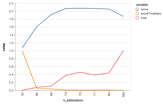
| n_estimators | score | time | scoreTimeRatio | |
|---|---|---|---|---|
| 0 | 32 | 1.073532 | 0.002459 | 1.000000 |
| 1 | 128 | 1.867858 | 1.002459 | 0.000000 |
| 2 | 80 | 2.052255 | 0.440060 | 0.006443 |
| 3 | 56 | 1.605447 | 0.075185 | 0.044843 |
| 4 | 68 | 1.910411 | 0.107187 | 0.036721 |
| 5 | 74 | 2.066440 | 0.377136 | 0.008320 |
| 6 | 77 | 2.066440 | 0.388378 | 0.007955 |
| 7 | 75 | 2.073532 | 0.457481 | 0.006141 |
| n_estimators | score | time | |
|---|---|---|---|
| 0 | 32 | 0.988663 | 0.180521 |
| 1 | 128 | 0.989403 | 0.587113 |
| 2 | 80 | 0.989575 | 0.358446 |
| 3 | 56 | 0.989159 | 0.210091 |
| 4 | 68 | 0.989443 | 0.223102 |
| 5 | 74 | 0.989588 | 0.332861 |
| 6 | 77 | 0.989588 | 0.337432 |
| 7 | 75 | 0.989595 | 0.365529 |
Hrm, looks like the score starts getting somewhere interesting around 68, and time starts shooting up at about 80. Let's do another with those as our bounds!
n_estimators = bgs.compareValsBaseCase(
    X,
    y,
    getForestAccuracy,
    rfArgs,
    "n_estimators",
    0,
    68,
    80
)

bgs.showTimeScoreChartAndGraph(n_estimators)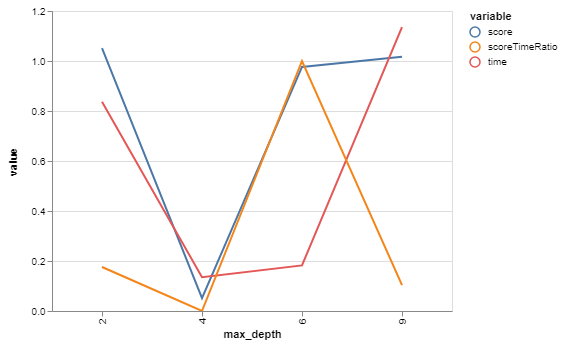
| n_estimators | score | time | scoreTimeRatio | |
|---|---|---|---|---|
| 0 | 68 | 6.390333 | 0.333407 | 0.135692 |
| 1 | 80 | 7.223667 | 1.064343 | 0.000000 |
| 2 | 74 | 7.307000 | 0.404471 | 0.123622 |
| 3 | 71 | 6.307000 | 0.064343 | 1.000000 |
| 4 | 72 | 6.390333 | 0.175190 | 0.325419 |
| n_estimators | score | time | |
|---|---|---|---|
| 0 | 68 | 0.989443 | 0.344220 |
| 1 | 80 | 0.989575 | 0.355580 |
| 2 | 74 | 0.989588 | 0.345324 |
| 3 | 71 | 0.989430 | 0.340038 |
| 4 | 72 | 0.989443 | 0.341761 |
71 looks like our winner! Or close enough for our purposes while we then go optimize other things. And we only had to train our model 13 times - as opposed to the 96 we would have with a brute-force grid search.
Hopefully this will become a series on using this to tune other RF hyperparameters - other ones have some interesting quirks that I'd like to expound upon. Or you could just look at the GitHub repo for spoilers. Or both!